Optimal Binary Search Tree Rytas 12/12/04
25 Slides356.00 KB
Optimal Binary Search Tree Rytas 12/12/04
1.Preface OBST is one special kind of advanced tree. It focus on how to reduce the cost of the search of the BST. It may not have the lowest height ! It needs 3 tables to record probabilities, cost, and root.
2.Premise It has n keys (representation k1,k2, ,kn) in sorted order (so that k1 k2 kn), and we wish to build a binary sear ch tree from these keys. For each ki ,we have a probabilit y pi that a search will be for ki. In contrast of, some searches may be for values not in ki, and so we also have n 1 “dummy keys” d0,d1, ,dn repre sentating not in ki. In particular, d0 represents all values less than k1, and dn represents all values greater than kn, and for i 1,2, ,n-1 , the dummy key di represents all values between ki and ki 1. * The dummy keys are leaves (external nodes), and th e data keys mean internal nodes.
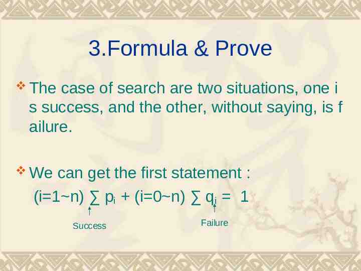
3.Formula & Prove The case of search are two situations, one i s success, and the other, without saying, is f ailure. We can get the first statement : (i 1 n) pi (i 0 n) qi 1 Success Failure
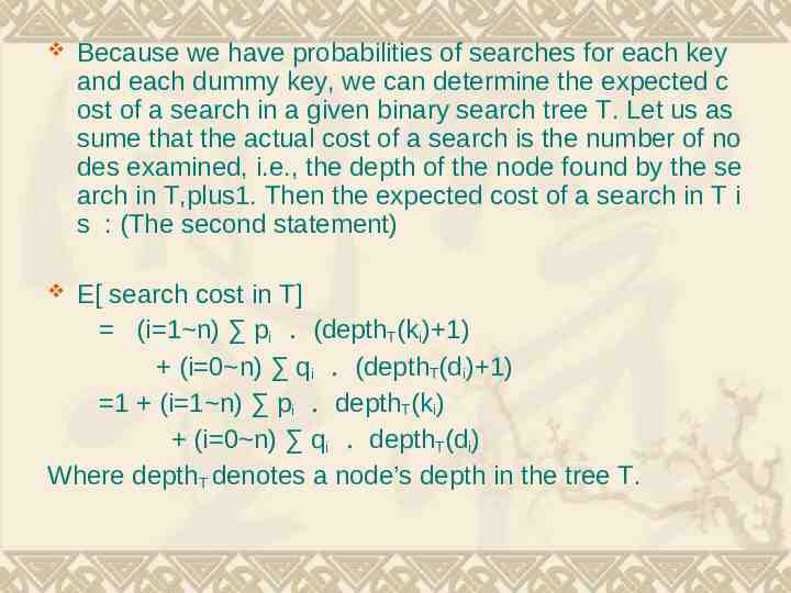
Because we have probabilities of searches for each key and each dummy key, we can determine the expected c ost of a search in a given binary search tree T. Let us as sume that the actual cost of a search is the number of no des examined, i.e., the depth of the node found by the se arch in T,plus1. Then the expected cost of a search in T i s : (The second statement) E[ search cost in T] (i 1 n) pi . (depthT(ki) 1) (i 0 n) qi . (depthT(di) 1) 1 (i 1 n) pi . depthT(ki) (i 0 n) qi . depthT(di) Where depthT denotes a node’s depth in the tree T.
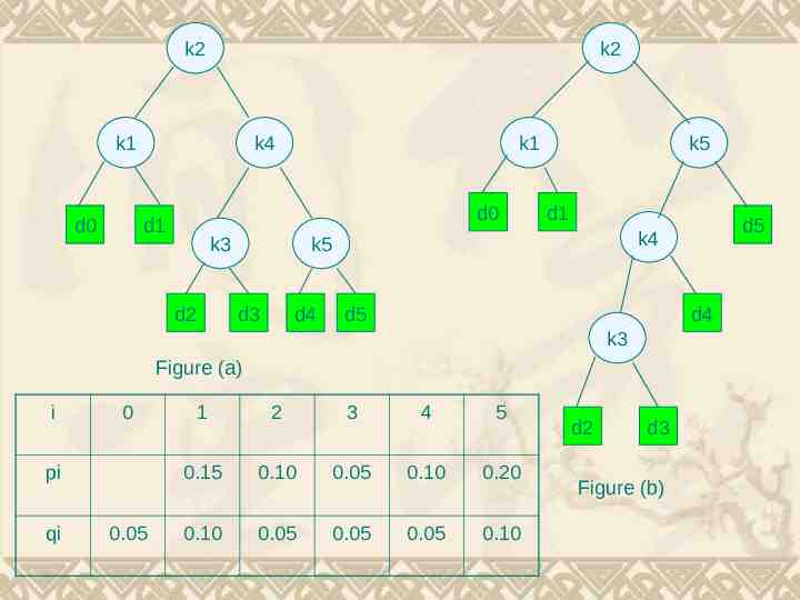
k2 k2 k1 d0 k4 k1 d0 d1 k3 d2 k5 d1 k5 d3 d4 d5 d4 k3 Figure (a) i 0 pi qi 0.05 d5 k4 1 2 3 4 5 0.15 0.10 0.05 0.10 0.20 0.10 0.05 0.05 0.05 0.10 d2 d3 Figure (b)
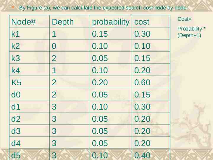
By Figure (a), we can calculate the expected search cost node by node: Node# k1 k2 k3 k4 K5 d0 d1 d2 d3 d4 d5 Depth 1 0 2 1 2 2 3 3 3 3 3 probability 0.15 0.10 0.05 0.10 0.20 0.05 0.10 0.05 0.05 0.05 0.10 cost 0.30 0.10 0.15 0.20 0.60 0.15 0.30 0.20 0.20 0.20 0.40 Cost Probability * (Depth 1)
And the total cost (0.30 0.10 0.15 0.20 0.60 0.15 0.30 0.20 0.20 0.20 0.40 ) 2.80 So Figure (a) costs 2.80 ,on another, the Figure (b) costs 2.75, and that tree is really optimal. We can see the height of (b) is more than (a) , and the key k5 has the greatest search probability of any key, yet the root of the OBST shown is k2.(The lowest expected cost of any BST with k5 at the root is 2.85)
Step1:The structure of an OBST To characterize the optimal substructu re of OBST, we start with an observatio n about subtrees. Consider any subtre e of a BST. It must contain keys in a co ntiguous range ki, ,kj, for some 1 i j n. In addition, a subtree that contai ns keys ki, ,kj must also have as its le aves the dummy keys di-1 , ,dj.
We need to use the optimal substructure to sho w that we can construct an optimal solution to th e problem from optimal solutions to subproblems . Given keys ki , , kj, one of these keys, say kr (I r j), will be the root of an optimal subtree cont aining these keys. The left subtree of the root kr will contain the keys (ki , , kr-1) and the dummy k eys( di-1 , , dr-1), and the right subtree will contai n the keys (kr 1 , , kj) and the dummy keys( dr , , dj). As long as we examine all candidate root s kr, where I r j, and we determine all optimal binary search trees containing ki , , kr-1 and thos e containing kr 1 , , kj , we are guaranteed that we will find an OBST.
There is one detail worth nothing about “empty” subtrees. Suppose that in a subtree with keys k i,.,kj, we select ki as the root. By the above argu ment, ki ‘s left subtree contains the keys ki, , ki-1 . It is natural to interpret this sequence as contai ning no keys. It is easy to know that subtrees als o contain dummy keys. The sequence has no ac tual keys but does contain the single dummy key di-1. Symmetrically, if we select kj as the root, the n kj‘s right subtree contains the keys, kj 1 ,kj; th is right subtree contains no actual keys, but it do es contain the dummy key dj.
Step2: A recursive solution We are ready to define the value of an optimal s olution recursively. We pick our subproblem dom ain as finding an OBST containing the keys ki, , kj, where i 1, j n, and j i-1. (It is when j i-1 t hat ther are no actual keys; we have just the du mmy key di-1.) Let us define e[i,j] as the expected cost of searc hing an OBST containing the keys ki, , kj. Ultim ately, we wish to compute e[1,n].
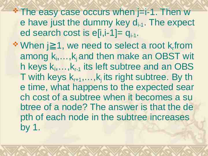
The easy case occurs when j i-1. Then w e have just the dummy key di-1. The expect ed search cost is e[i,i-1] qi-1. When j 1, we need to select a root krfrom among ki, ,kj and then make an OBST wit h keys ki, ,kr-1 its left subtree and an OBS T with keys kr 1, ,kj its right subtree. By th e time, what happens to the expected sear ch cost of a subtree when it becomes a su btree of a node? The answer is that the de pth of each node in the subtree increases by 1.
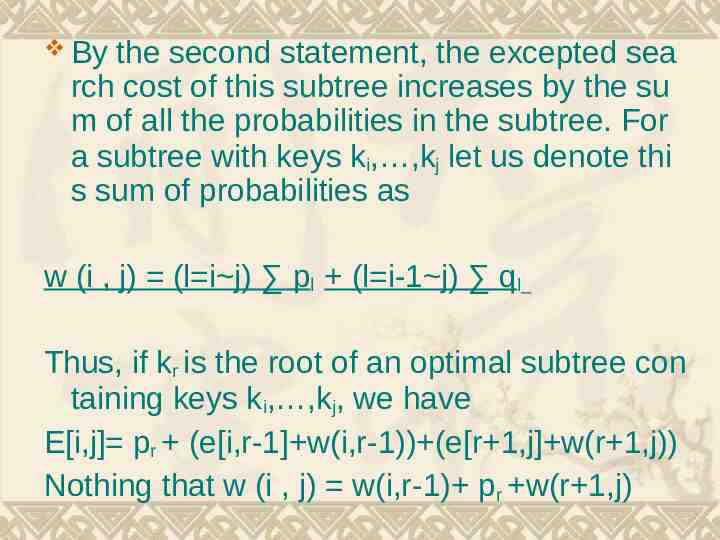
By the second statement, the excepted sea rch cost of this subtree increases by the su m of all the probabilities in the subtree. For a subtree with keys ki, ,kj let us denote thi s sum of probabilities as w (i , j) (l i j) pl (l i-1 j) ql Thus, if kr is the root of an optimal subtree con taining keys ki, ,kj, we have E[i,j] pr (e[i,r-1] w(i,r-1)) (e[r 1,j] w(r 1,j)) Nothing that w (i , j) w(i,r-1) pr w(r 1,j)
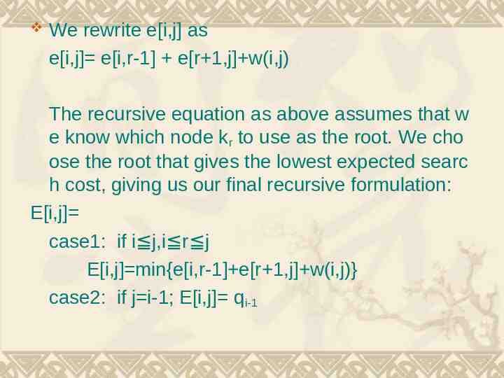
We rewrite e[i,j] as e[i,j] e[i,r-1] e[r 1,j] w(i,j) The recursive equation as above assumes that w e know which node kr to use as the root. We cho ose the root that gives the lowest expected searc h cost, giving us our final recursive formulation: E[i,j] case1: if i j,i r j E[i,j] min{e[i,r-1] e[r 1,j] w(i,j)} case2: if j i-1; E[i,j] qi-1
The e[i,j] values give the expected search costs in OBST. To help us keep track of th e structure of OBST, we define root[i,j], for 1 i j n, to be the index r for which kr is t he root of an OBST containing keys ki, ,kj .
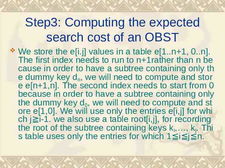
Step3: Computing the expected search cost of an OBST We store the e[i.j] values in a table e[1.n 1, 0.n]. The first index needs to run to n 1rather than n be cause in order to have a subtree containing only th e dummy key dn, we will need to compute and stor e e[n 1,n]. The second index needs to start from 0 because in order to have a subtree containing only the dummy key d0, we will need to compute and st ore e[1,0]. We will use only the entries e[i,j] for whi ch j i-1. we also use a table root[i,j], for recording the root of the subtree containing keys k i, , kj. Thi s table uses only the entries for which 1 i j n.
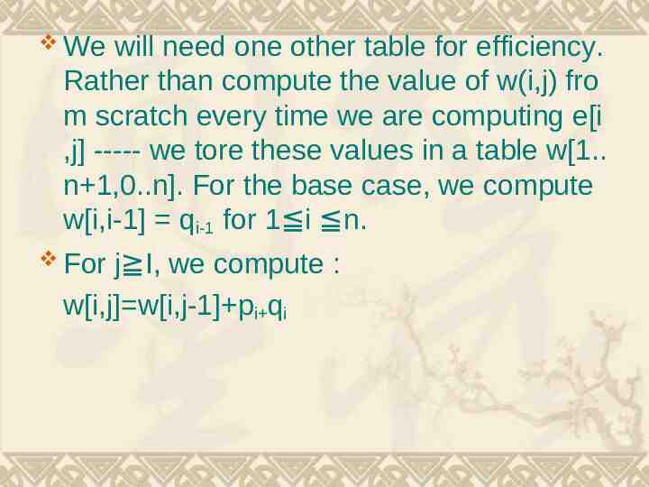
We will need one other table for efficiency. Rather than compute the value of w(i,j) fro m scratch every time we are computing e[i ,j] ----- we tore these values in a table w[1. n 1,0.n]. For the base case, we compute w[i,i-1] qi-1 for 1 i n. j I, we compute : w[i,j] w[i,j-1] pi qi For
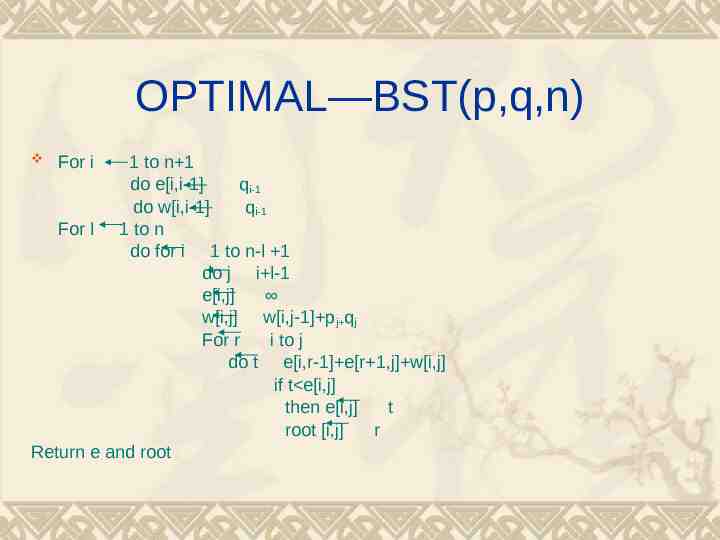
OPTIMAL—BST(p,q,n) 1 to n 1 do e[i,i-1] qi-1 do w[i,i-1] qi-1 For l 1 to n do for i 1 to n-l 1 do j i l-1 e[i,j] w[i,j] w[i,j-1] pj qj For r i to j do t e[i,r-1] e[r 1,j] w[i,j] if t e[i,j] then e[i,j] t root [i,j] r Return e and root For i
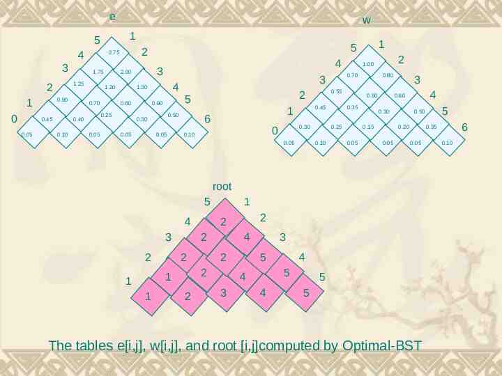
e 1 5 3 0.45 0.05 1.75 0.90 1 0 4 1.20 0.70 0.10 0.05 4 1.30 0.60 0.25 0.40 4 3 2.00 0.90 0.05 0.55 2 5 0.45 1 6 0.30 0 0.10 0.05 0.80 0.50 0.35 0.25 0.10 2 1.00 0.70 3 0.50 0.30 0.05 1 5 2 2.75 1.25 2 w 4 0.60 0.30 0.15 0.05 3 0.20 0.05 4 0.05 3 2 2 2 1 2 2 4 2 2 1 1 1 2 3 5 3 4 5 4 4 6 0.35 root 5 5 0.50 5 5 The tables e[i,j], w[i,j], and root [i,j]computed by Optimal-BST 0.10
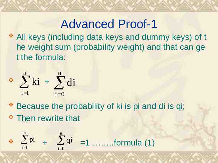
Advanced Proof-1 All keys (including data keys and dummy keys) of t he weight sum (probability weight) and that can ge t the formula: n n i 1 i 0 ki di Because the probability of ki is pi and di is qi; Then rewrite that n pi i 1 n qi i 0 1 .formula (1)
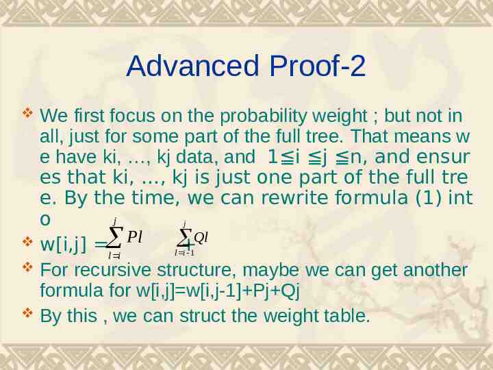
Advanced Proof-2 We first focus on the probability weight ; but not in all, just for some part of the full tree. That means w e have ki, , kj data, and 1 i j n, and ensur es that ki, , kj is just one part of the full tre e. By the time, we can rewrite formula (1) int j o j Ql w[i,j] Pl l i 1 l i For recursive structure, maybe we can get another formula for w[i,j] w[i,j-1] Pj Qj By this , we can struct the weight table.
Advanced Proof-3 Finally, we want to discuss our topic, without saying, the cost, which is expected to be the optimal one. Then define the recursive structure’s cost e[i ,j], which means ki, , kj, 1 i j n, cost. And we can divide into root, leftsubtre e, and rightsubtree.
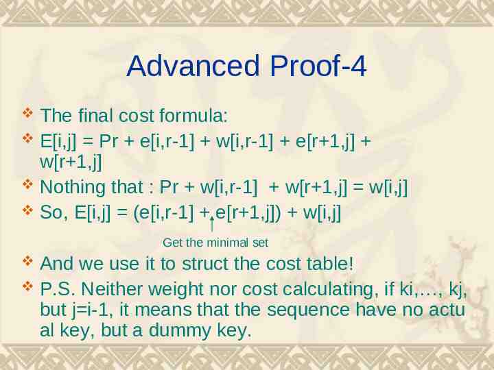
Advanced Proof-4 The final cost formula: E[i,j] Pr e[i,r-1] w[i,r-1] e[r 1,j] w[r 1,j] Nothing that : Pr w[i,r-1] w[r 1,j] w[i,j] So, E[i,j] (e[i,r-1] e[r 1,j]) w[i,j] Get the minimal set And we use it to struct the cost table! P.S. Neither weight nor cost calculating, if ki, , kj, but j i-1, it means that the sequence have no actu al key, but a dummy key.
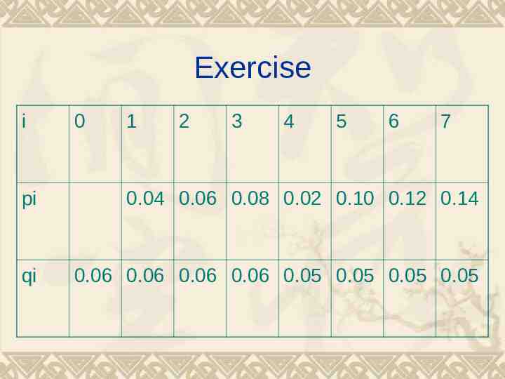
Exercise i 0 1 2 3 4 5 6 7 pi 0.04 0.06 0.08 0.02 0.10 0.12 0.14 qi 0.06 0.06 0.06 0.06 0.05 0.05 0.05 0.05