NESC ACADEMY WEBCAST An Alternate Damage Potential Method
51 Slides8.22 MB
NESC ACADEMY WEBCAST An Alternate Damage Potential Method for Enveloping Nonstationary Random Vibration Tom Irvine Dynamic Concepts, Inc Email: [email protected] Learning from the Past, Looking to the Future Page: 1
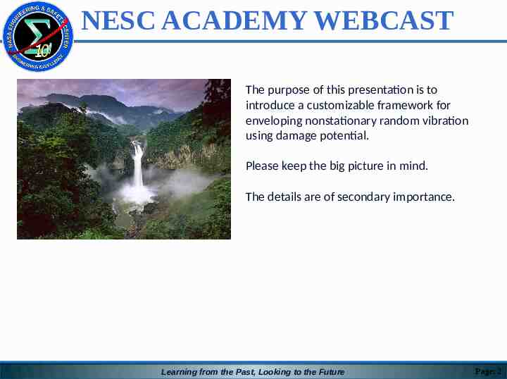
NESC ACADEMY WEBCAST The purpose of this presentation is to introduce a customizable framework for enveloping nonstationary random vibration using damage potential. Please keep the big picture in mind. The details are of secondary importance. Learning from the Past, Looking to the Future Page: 2
NESC ACADEMY WEBCAST This project is an informal collaboration between: NESC NASA KSC Dynamic Concepts Space-X In the Spirit of the National Aeronautics and Space Act of 1958 Falcon 9 Liftoff Learning from the Past, Looking to the Future Page: 3
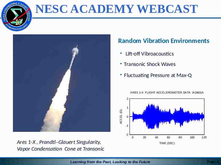
NESC ACADEMY WEBCAST Random Vibration Environments Lift-off Vibroacoustics Transonic Shock Waves Fluctuating Pressure at Max-Q ARES 1-X FLIGHT ACCELEROMETER DATA IAD601A 2 ACCEL (G) 1 0 -1 -2 0 20 Ares 1-X , Prandtl–Glauert Singularity, Vapor Condensation Cone at Transonic Learning from the Past, Looking to the Future 40 60 80 100 120 TIME (SEC) Page: 4
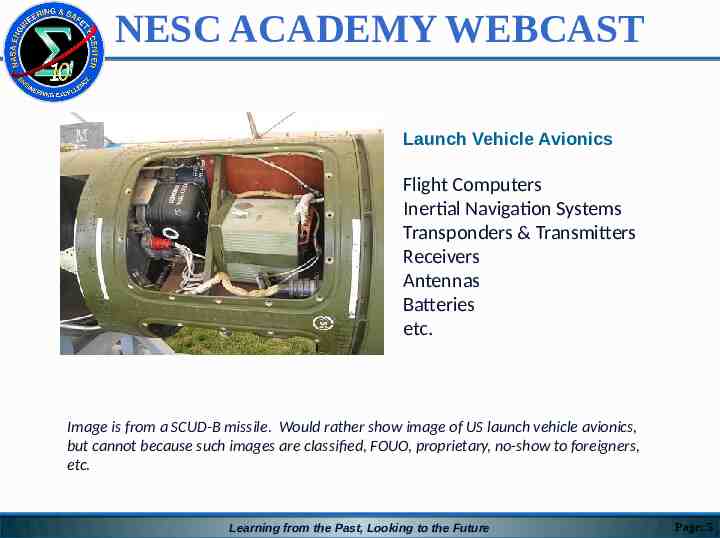
NESC ACADEMY WEBCAST Launch Vehicle Avionics Flight Computers Inertial Navigation Systems Transponders & Transmitters Receivers Antennas Batteries etc. Image is from a SCUD-B missile. Would rather show image of US launch vehicle avionics, but cannot because such images are classified, FOUO, proprietary, no-show to foreigners, etc. Learning from the Past, Looking to the Future Page: 5
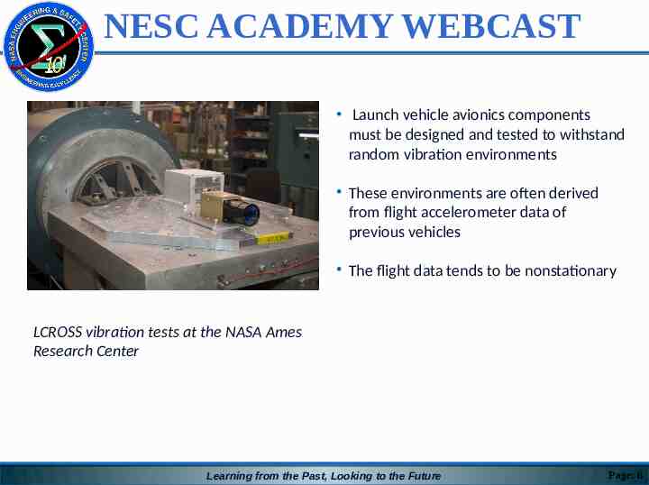
NESC ACADEMY WEBCAST Launch vehicle avionics components must be designed and tested to withstand random vibration environments These environments are often derived from flight accelerometer data of previous vehicles The flight data tends to be nonstationary LCROSS vibration tests at the NASA Ames Research Center Learning from the Past, Looking to the Future Page: 6
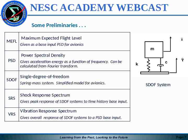
NESC ACADEMY WEBCAST Some Preliminaries . . . MEFL Maximum Expected Flight Level Given as a base input PSD for avionics Power Spectral Density PSD SDOF SRS VRS Gives acceleration energy as a function of frequency. Can be calculated from Fourier transform. Single-degree-of-freedom Spring-mass system. Simplified model for avionics. SDOF System Shock Response Spectrum Gives peak response of SDOF systems to time history base input. Vibration Response Spectrum Gives overall response of SDOF systems to a PSD base input. Learning from the Past, Looking to the Future Page: 7
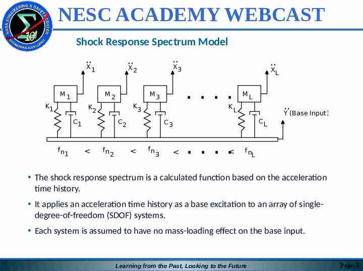
NESC ACADEMY WEBCAST Shock Response Spectrum Model . M1 K 3 C1 fn 1 fn 2 ML Y (Base Input) CL C3 . KL C2 XL . M3 K2 . X3 X2 M2 K 1 . . X1 fn 3 . fn L The shock response spectrum is a calculated function based on the acceleration time history. It applies an acceleration time history as a base excitation to an array of singledegree-of-freedom (SDOF) systems. Each system is assumed to have no mass-loading effect on the base input. Learning from the Past, Looking to the Future Page: 8
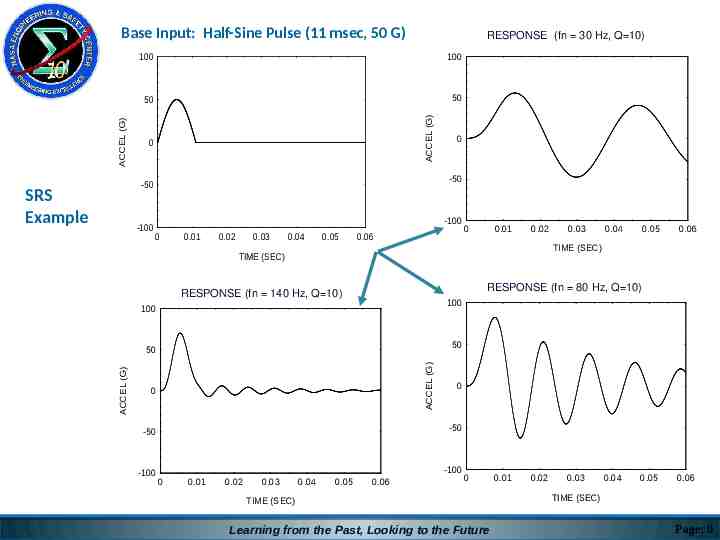
NESC ACADEMY WEBCAST RESPONSE (fn 30 Hz, Q 10) 100 100 50 50 ACCEL (G) ACCEL (G) Base Input: Half-Sine Pulse (11 msec, 50 G) 0 -50 -50 SRS Example -100 0 -100 0 0.01 0.02 0.03 0.04 0.05 0.06 0 0.01 0.02 0.05 0.06 RESPONSE (fn 80 Hz, Q 10) RESPONSE (fn 140 Hz, Q 10) 100 100 50 ACCEL (G) 50 ACCEL (G) 0.04 TIME (SEC) TIME (SEC) 0 0 -50 -50 -100 0.03 -100 0 0.01 0.02 0.03 0.04 0.05 0.06 0 TIME (SEC) Learning from the Past, Looking to the Future 0.01 0.02 0.03 0.04 0.05 0.06 TIME (SEC) Page: 9
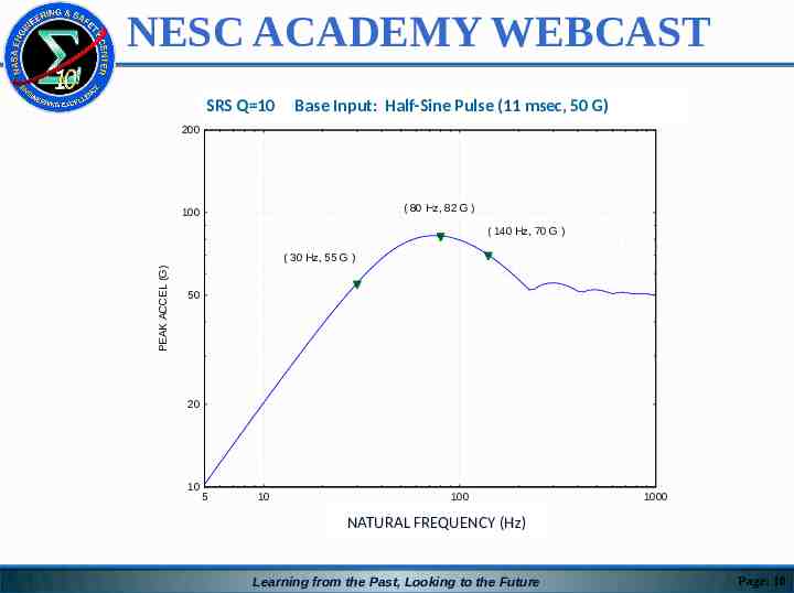
NESC ACADEMY WEBCAST Q 10 Input: BASE INPUT: HALF-SINE PULSE (11 msec, msec, 50 50 G) G) SRS Q 10SRSBase Half-Sine Pulse (11 200 ( 80 Hz, 82 G ) 100 ( 140 Hz, 70 G ) PEAK ACCEL (G) ( 30 Hz, 55 G ) 50 20 10 5 10 100 1000 NATURAL FREQUENCY (Hz)(Hz) NATURAL FREQUENCY Learning from the Past, Looking to the Future Page: 10
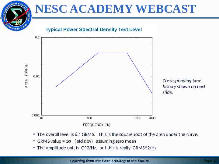
NESC ACADEMY WEBCAST Typical Power Spectral Density Test Level 2 ACCEL (G /Hz) 0.1 0.01 Corresponding time history shown on next slide. 0.001 10 100 1000 2000 FREQUENCY (Hz) The overall level is 6.1 GRMS. This is the square root of the area under the curve. GRMS value 1s ( std dev) assuming zero mean The amplitude unit is G 2/Hz, but this is really GRMS 2/Hz Learning from the Past, Looking to the Future Page: 11
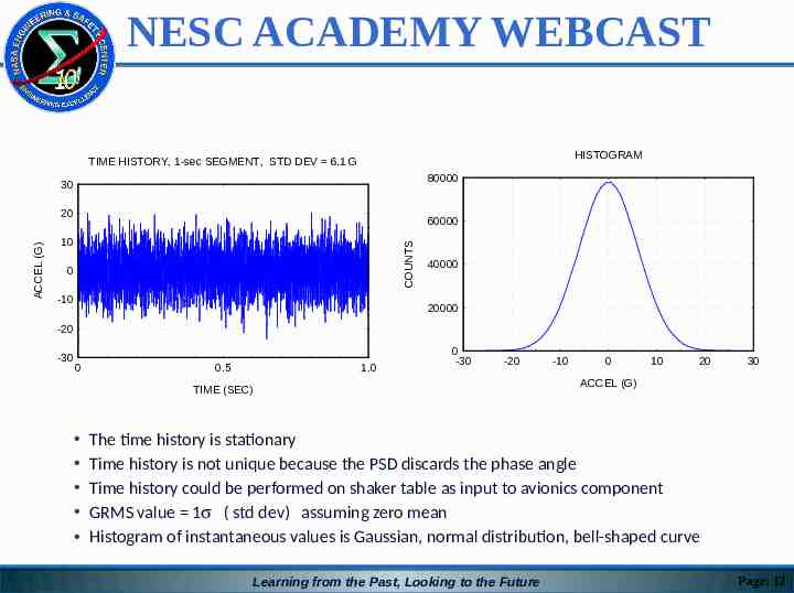
NESC ACADEMY WEBCAST HISTOGRAM TIME HISTORY, 1-sec SEGMENT, STD DEV 6.1 G 80000 30 60000 10 COUNTS ACCEL (G) 20 0 -10 40000 20000 -20 -30 0 0.5 1.0 0 -30 -20 TIME (SEC) -10 0 10 20 30 ACCEL (G) The time history is stationary Time history is not unique because the PSD discards the phase angle Time history could be performed on shaker table as input to avionics component GRMS value 1s ( std dev) assuming zero mean Histogram of instantaneous values is Gaussian, normal distribution, bell-shaped curve Learning from the Past, Looking to the Future Page: 12
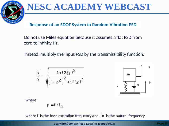
NESC ACADEMY WEBCAST Response of an SDOF System to Random Vibration PSD Do not use Miles equation because it assumes a flat PSD from zero to infinity Hz. Instead, multiply the input PSD by the transmissibility function: x y where 1 2 2 2 2 1 2 2 f / f n where f is the base excitation frequency and fn is the natural frequency. Learning from the Past, Looking to the Future Page: 13
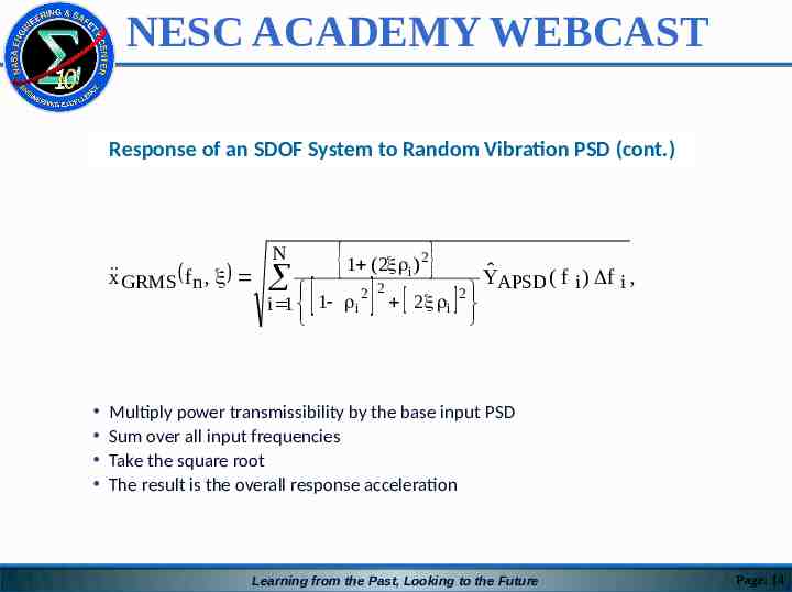
NESC ACADEMY WEBCAST Response of an SDOF System to Random Vibration PSD (cont.) x GRMS f n , N 1 (2 ) i i 1 1 i 2 2 2 2 i 2 ŶAPSD ( f i ) f i , Multiply power transmissibility by the base input PSD Sum over all input frequencies Take the square root The result is the overall response acceleration Learning from the Past, Looking to the Future Page: 14
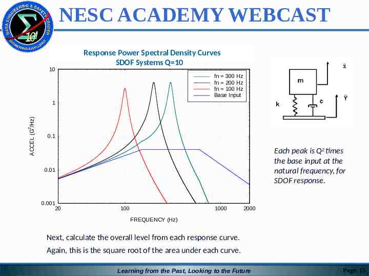
NESC ACADEMY WEBCAST 10 Response Power Spectral Density Curves SDOF Systems Q 10 fn 300 Hz fn 200 Hz fn 100 Hz Base Input 2 ACCEL (G /Hz) 1 0.1 Each peak is Q2 times the base input at the natural frequency, for SDOF response. 0.01 0.001 20 100 1000 2000 FREQUENCY (Hz) Next, calculate the overall level from each response curve. Again, this is the square root of the area under each curve. Learning from the Past, Looking to the Future Page: 15
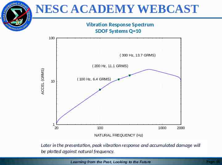
NESC ACADEMY WEBCAST Vibration Response Spectrum SDOF Systems Q 10 100 ( 300 Hz, 13.7 GRMS) ACCEL (GRMS) ( 200 Hz, 11.1 GRMS) 10 1 20 ( 100 Hz, 6.4 GRMS) 100 1000 2000 NATURAL FREQUENCY (Hz) Later in the presentation, peak vibration response and accumulated damage will be plotted against natural frequency. Learning from the Past, Looking to the Future Page: 16
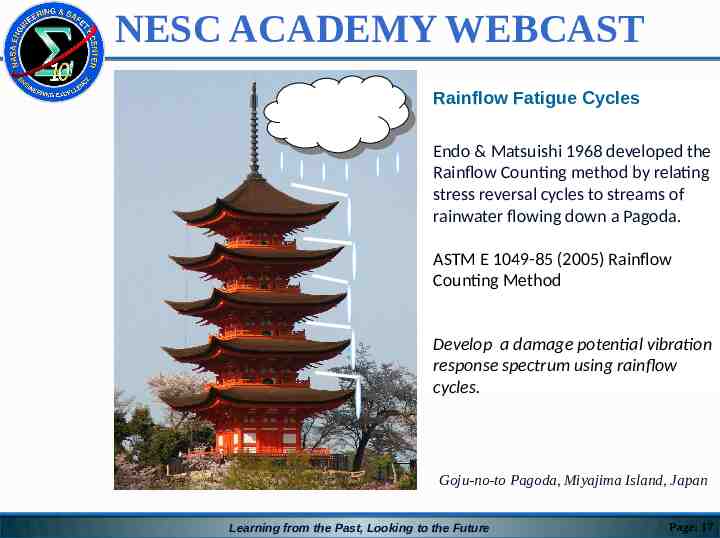
NESC ACADEMY WEBCAST Rainflow Fatigue Cycles Endo & Matsuishi 1968 developed the Rainflow Counting method by relating stress reversal cycles to streams of rainwater flowing down a Pagoda. ASTM E 1049-85 (2005) Rainflow Counting Method Develop a damage potential vibration response spectrum using rainflow cycles. Goju-no-to Pagoda, Miyajima Island, Japan Learning from the Past, Looking to the Future Page: 17
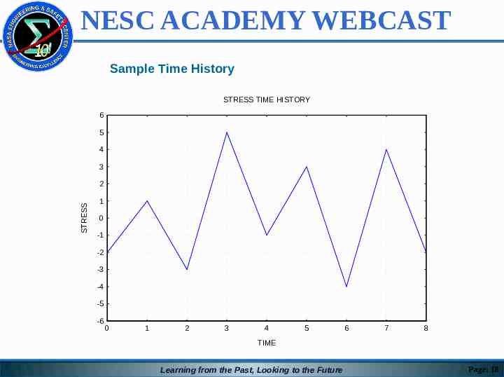
NESC ACADEMY WEBCAST Sample Time History STRESS TIME HISTORY 6 5 4 3 STRESS 2 1 0 -1 -2 -3 -4 -5 -6 0 1 2 3 4 5 6 7 8 TIME Learning from the Past, Looking to the Future Page: 18
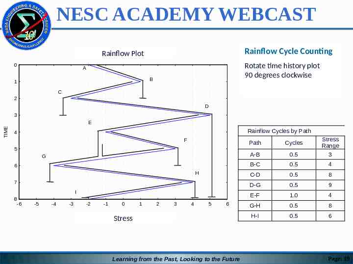
NESC ACADEMY WEBCAST Rainflow Cycle Counting Rainflow Plot RAINFLOW PLOT 0 Rotate time history plot 90 degrees clockwise A B 1 C 2 D 3 TIME E Rainflow Cycles by Path 4 F 5 G 6 H 7 I 8 -6 -5 -4 -3 -2 -1 0 1 2 3 4 5 6 STRESS Stress Learning from the Past, Looking to the Future Path Cycles A-B 0.5 Stress Range 3 B-C 0.5 4 C-D 0.5 8 D-G 0.5 9 E-F 1.0 4 G-H 0.5 8 H-I 0.5 6 Page: 19
NESC ACADEMY WEBCAST Derive MEFL from Nonstationary Random Vibration The typical method for post-processing is to divide the data into short-duration segments The segments may overlap This is termed piecewise stationary analysis A PSD is then taken for each segment The maximum envelope is then taken from the individual PSD curves MEFL maximum envelope some uncertainty margin Component acceptance test level MEFL Easy to do But potentially overly conservative Learning from the Past, Looking to the Future Page: 20
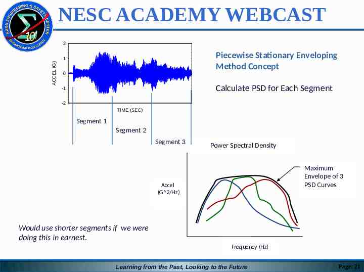
NESC ACADEMY WEBCAST 2 Piecewise Stationary Enveloping Method Concept ACCEL (G) 1 0 Calculate PSD for Each Segment -1 -2 TIME (SEC) Segment 1 Segment 2 Segment 3 Power Spectral Density Maximum Envelope of 3 PSD Curves Accel (G 2/Hz) Would use shorter segments if we were doing this in earnest. Frequency (Hz) Learning from the Past, Looking to the Future Page: 21
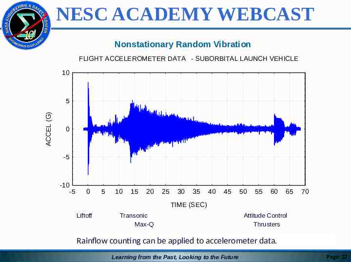
NESC ACADEMY WEBCAST Nonstationary Random Vibration FLIGHT ACCELEROMETER DATA - SUBORBITAL LAUNCH VEHICLE 10 ACCEL (G) 5 0 -5 -10 -5 0 5 10 15 20 25 30 35 40 45 50 55 60 65 70 TIME (SEC) Liftoff Transonic Max-Q Attitude Control Thrusters Rainflow counting can be applied to accelerometer data. Learning from the Past, Looking to the Future Page: 22
NESC ACADEMY WEBCAST Background Reference S. J. DiMaggio, B. H. Sako, and S. Rubin, Analysis of Nonstationary Vibroacoustic Flight Data Using a Damage-Potential Basis, Journal of Spacecraft and Rockets, Vol, 40, No. 5. September-October 2003. This is a brilliant paper but requires a Ph.D. in statistics to understand. Need a more accessible method for the journeyman vibration analyst, along with a set of shareable software programs, including source code Use same overall approach as DiMaggio, Sako & Rubin, but fill in the details using brute-force numerical simulation Alternate method will be easy-to-understand but bookkeeping-intensive But software does the bookkeeping Learning from the Past, Looking to the Future Page: 23
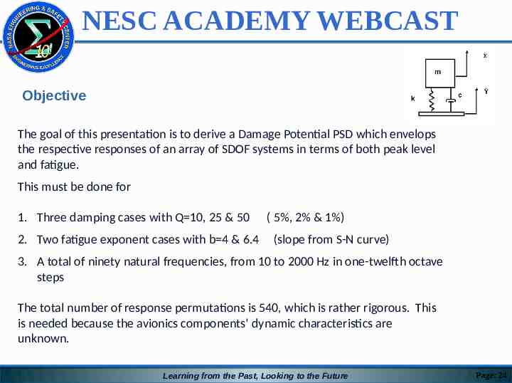
NESC ACADEMY WEBCAST Objective The goal of this presentation is to derive a Damage Potential PSD which envelops the respective responses of an array of SDOF systems in terms of both peak level and fatigue. This must be done for 1. Three damping cases with Q 10, 25 & 50 2. Two fatigue exponent cases with b 4 & 6.4 ( 5%, 2% & 1%) (slope from S-N curve) 3. A total of ninety natural frequencies, from 10 to 2000 Hz in one-twelfth octave steps The total number of response permutations is 540, which is rather rigorous. This is needed because the avionics components’ dynamic characteristics are unknown. Learning from the Past, Looking to the Future Page: 24
NESC ACADEMY WEBCAST Objective (cont.) The alternate damage method in this paper builds upon previous work by addressing an additional concern as follows: 1. Consider an SDOF system with a given natural frequency and damping ratio 2. The SDOF system is subjected to a base input 3. The base input may vary significantly with frequency 4. The response of the SDOF system may include non-resonant stress reversal cycles Learning from the Past, Looking to the Future Page: 25
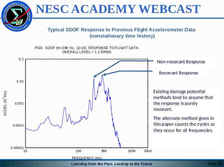
NESC ACADEMY WEBCAST Typical SDOF Response to Previous Flight Accelerometer Data (nonstationary time history) PSD SDOF (fn 280 Hz, Q 10) RESPONSE TO FLIGHT DATA OVERALL LEVEL 1.1 GRMS 0.1 Non-resonant Response Resonant Response Existing damage potential methods tend to assume that the response is purely resonant. 2 ACCEL (G /Hz) 0.01 0.001 The alternate method given in this paper counts the cycles as they occur for all frequencies. 0.0001 0.00001 10 100 300 1000 2000 FREQUENCY (Hz) Learning from the Past, Looking to the Future Page: 26
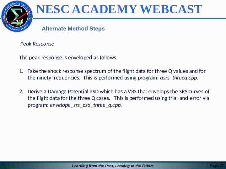
NESC ACADEMY WEBCAST Alternate Method Steps Peak Response The peak response is enveloped as follows. 1. Take the shock response spectrum of the flight data for three Q values and for the ninety frequencies. This is performed using program: qsrs threeq.cpp. 2. Derive a Damage Potential PSD which has a VRS that envelops the SRS curves of the flight data for the three Q cases. This is performed using trial-and-error via program: envelope srs psd three q.cpp. Learning from the Past, Looking to the Future Page: 27
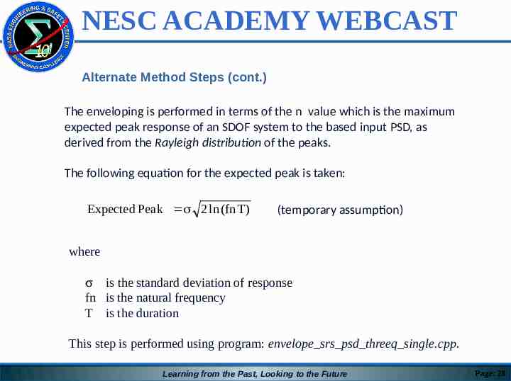
NESC ACADEMY WEBCAST Alternate Method Steps (cont.) The enveloping is performed in terms of the n value which is the maximum expected peak response of an SDOF system to the based input PSD, as derived from the Rayleigh distribution of the peaks. The following equation for the expected peak is taken: Expected Peak 2 ln (fn T) (temporary assumption) where s is the standard deviation of response fn is the natural frequency T is the duration This step is performed using program: envelope srs psd threeq single.cpp. Learning from the Past, Looking to the Future Page: 28
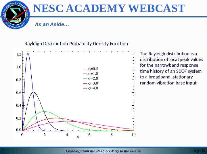
NESC ACADEMY WEBCAST As an Aside Rayleigh Distribution Probability Density Function The Rayleigh distribution is a distribution of local peak values for the narrowband response time history of an SDOF system to a broadband, stationary, random vibration base input Learning from the Past, Looking to the Future Page: 29
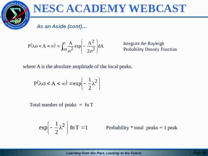
NESC ACADEMY WEBCAST As an Aside (cont) A2 A dA P A exp 2 2 2 Integrate the Rayleigh Probability Density Function where A is the absolute amplitude of the local peaks. 1 P A exp 2 2 Total number of peaks fn T 1 exp 2 fn T 1 2 Probability * total peaks 1 peak Learning from the Past, Looking to the Future Page: 30
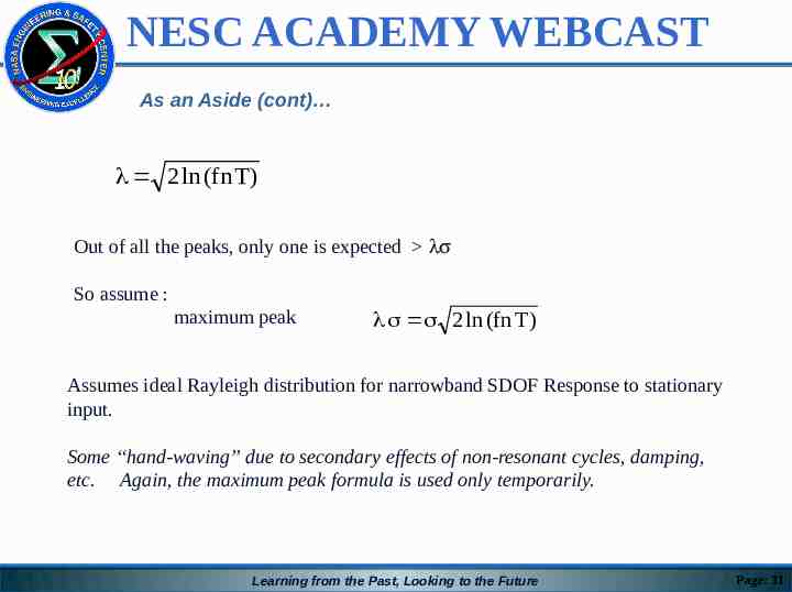
NESC ACADEMY WEBCAST As an Aside (cont) 2 ln (fn T) Out of all the peaks, only one is expected ls So assume : maximum peak 2 ln (fn T) Assumes ideal Rayleigh distribution for narrowband SDOF Response to stationary input. Some “hand-waving” due to secondary effects of non-resonant cycles, damping, etc. Again, the maximum peak formula is used only temporarily. Learning from the Past, Looking to the Future Page: 31
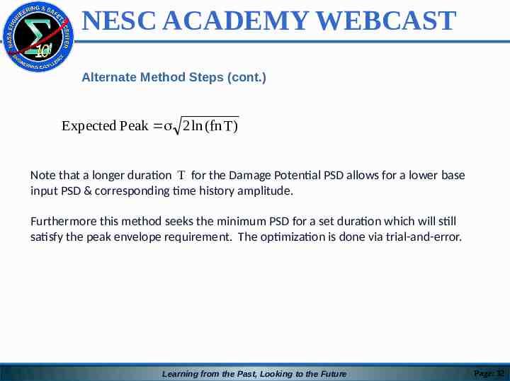
NESC ACADEMY WEBCAST Alternate Method Steps (cont.) Expected Peak 2 ln (fn T) Note that a longer duration T for the Damage Potential PSD allows for a lower base input PSD & corresponding time history amplitude. Furthermore this method seeks the minimum PSD for a set duration which will still satisfy the peak envelope requirement. The optimization is done via trial-and-error. Learning from the Past, Looking to the Future Page: 32
NESC ACADEMY WEBCAST Alternate Method Steps (cont.) Fatigue Check* The peak response criterion tends to be more stringent than the fatigue requirement. But fatigue damage should be verified for thoroughness. The fatigue damage for the Damage Potential PSD is performed as follows. Synthesize a time history to satisfy the Damage-Potential PSD. This is performed using program: psdgen.cpp. The time history is non-unique because the PSD discards phase angles. Calculate the time domain response for each of the three Q values and at each of the ninety natural frequencies. This is performed using program: arbit threeq.cpp. * This is not “true fatigue” which would be calculated from stress. Rather it is a fatiguelike metric for accumulated response acceleration cycles. Learning from the Past, Looking to the Future Page: 33
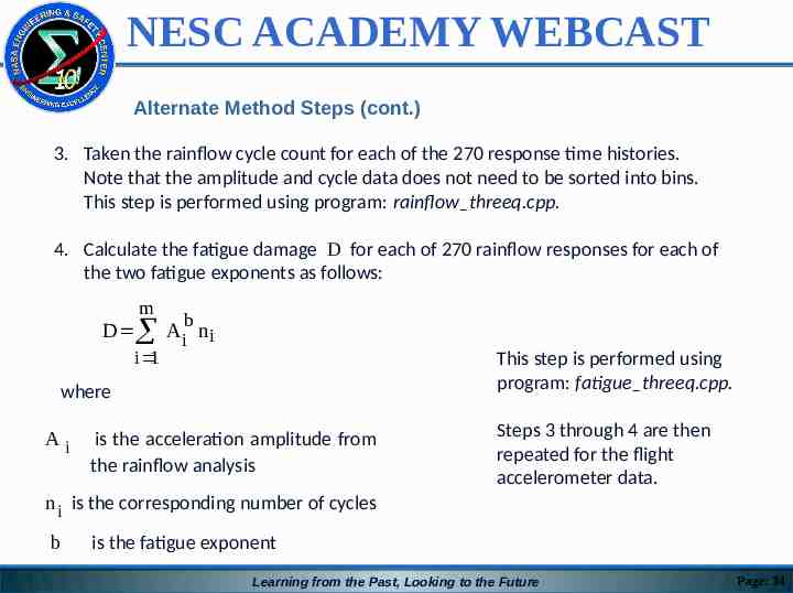
NESC ACADEMY WEBCAST Alternate Method Steps (cont.) 3. Taken the rainflow cycle count for each of the 270 response time histories. Note that the amplitude and cycle data does not need to be sorted into bins. This step is performed using program: rainflow threeq.cpp. 4. Calculate the fatigue damage D for each of 270 rainflow responses for each of the two fatigue exponents as follows: m b D Ai n i i 1 This step is performed using program: fatigue threeq.cpp. where Ai is the acceleration amplitude from the rainflow analysis Steps 3 through 4 are then repeated for the flight accelerometer data. n i is the corresponding number of cycles b is the fatigue exponent Learning from the Past, Looking to the Future Page: 34
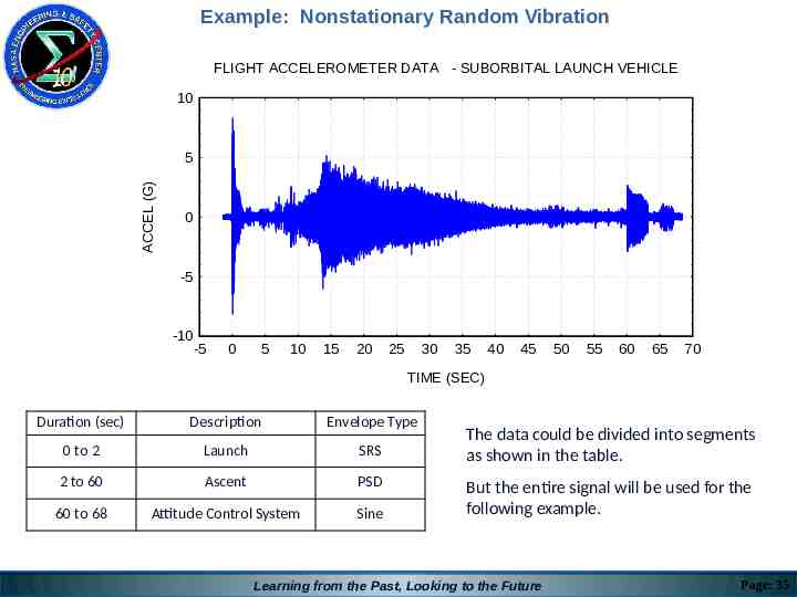
Example: Nonstationary Random Vibration NESC ACADEMY WEBCAST FLIGHT ACCELEROMETER DATA - SUBORBITAL LAUNCH VEHICLE 10 ACCEL (G) 5 0 -5 -10 -5 0 5 10 15 20 25 30 35 40 45 50 55 60 65 70 TIME (SEC) Duration (sec) Description Envelope Type 0 to 2 Launch SRS 2 to 60 Ascent PSD 60 to 68 Attitude Control System Sine The data could be divided into segments as shown in the table. But the entire signal will be used for the following example. Learning from the Past, Looking to the Future Page: 35
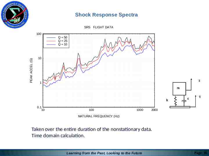
NESC ACADEMY WEBCAST Shock Response Spectra SRS FLIGHT DATA 100 PEAK ACCEL (G) Q 50 Q 25 Q 10 10 1 0.1 10 100 1000 2000 NATURAL FREQUENCY (Hz) Taken over the entire duration of the nonstationary data. Time domain calculation. Learning from the Past, Looking to the Future Page: 36
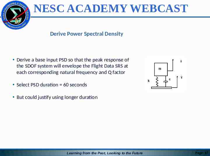
NESC ACADEMY WEBCAST Derive Power Spectral Density Derive a base input PSD so that the peak response of the SDOF system will envelope the Flight Data SRS at each corresponding natural frequency and Q factor Select PSD duration 60 seconds But could justify using longer duration Learning from the Past, Looking to the Future Page: 37
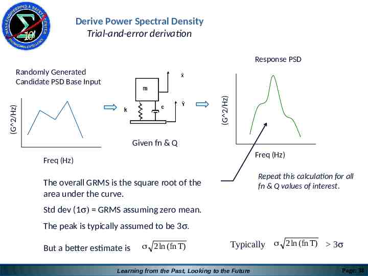
NESC ACADEMY WEBCAST Derive Power Spectral Density Trial-and-error derivation Response PSD (G 2/Hz) (G 2/Hz) Randomly Generated Candidate PSD Base Input Given fn & Q Freq (Hz) Freq (Hz) Repeat this calculation for all fn & Q values of interest. The overall GRMS is the square root of the area under the curve. Std dev (1s) GRMS assuming zero mean. The peak is typically assumed to be 3s. But a better estimate is 2 ln (fn T ) Typically 2 ln (fn T) 3s Learning from the Past, Looking to the Future Page: 38
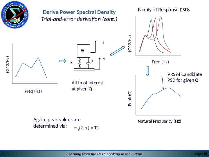
Family of Response PSDs NESC ACADEMY WEBCAST Derive Power Spectral Density (G 2/Hz) (G 2/Hz) Trial-and-error derivation (cont.) Freq (Hz) Again, peak values are determined via: 2 ln (fn T) Peak (G) Freq (Hz) All fn of interest at given Q VRS of Candidate PSD for given Q Natural Frequency (Hz) Learning from the Past, Looking to the Future Page: 39
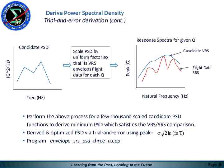
NESC ACADEMY WEBCAST Derive Power Spectral Density Trial-and-error derivation (cont.) Response Spectra for given Q Freq (Hz) Scale PSD by uniform factor so that its VRS envelops flight data for each Q Candidate VRS Peak (G) (G 2/Hz) Candidate PSD Flight Data SRS Natural Frequency (Hz) Perform the above process for a few thousand scaled candidate PSD functions to derive minimum PSD which satisfies the VRS/SRS comparison. Derived & optimized PSD via trial-and-error using peak 2 ln (fn T) Program: envelope srs psd three q.cpp Learning from the Past, Looking to the Future Page: 40
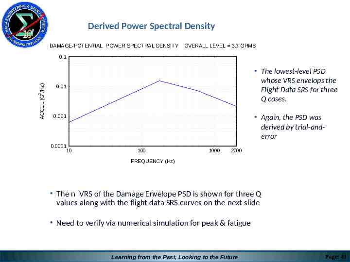
NESC ACADEMY WEBCAST Derived Power Spectral Density DAMAGE-POTENTIAL POWER SPECTRAL DENSITY OVERALL LEVEL 3.3 GRMS The lowest-level PSD whose VRS envelops the Flight Data SRS for three Q cases. 0.01 2 ACCEL (G /Hz) 0.1 Again, the PSD was derived by trial-anderror 0.001 0.0001 10 100 1000 2000 FREQUENCY (Hz) The n VRS of the Damage Envelope PSD is shown for three Q values along with the flight data SRS curves on the next slide Need to verify via numerical simulation for peak & fatigue Learning from the Past, Looking to the Future Page: 41
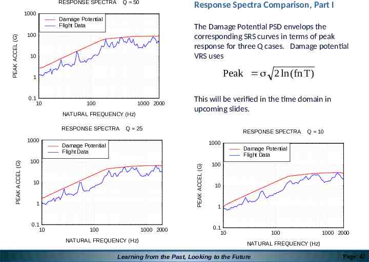
Response WEBCAST NESC ACADEMY ResponseSpectra SpectraComparison, Comparison,Part PartII RESPONSE SPECTRA PEAK ACCEL (G) 1000 Q 50 Response Spectra Comparison, Part I The Damage PSD envelops the the The DamagePotential Potential PSD envelops corresponding SRS curves in terms of peak corresponding SRS curves in terms of peak response for three Q cases. Damage potential response for three Q cases. Damage VRS uses VRS uses potential Damage Potential Flight Data 100 10 Peak 2 ln (fn T) 1 0.1 10 100 1000 2000 NATURAL FREQUENCY (Hz) RESPONSE SPECTRA Q 25 1000 Damage Potential Flight Data 100 10 1 0.1 10 RESPONSE SPECTRA PEAK ACCEL (G) PEAK ACCEL (G) 1000 This willbebeverified verified in the domain This will in the timetime domain in in upcoming slides. upcoming slides. 100 1000 2000 NATURAL FREQUENCY (Hz) Q 10 Damage Potential Flight Data 100 10 1 0.1 10 100 1000 2000 NATURAL FREQUENCY (Hz) Learning from the Past, Looking to the Future Page: 42
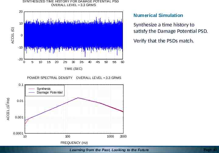
NESC ACADEMY WEBCAST SYNTHESIZED TIME HISTORY FOR DAMAGE POTENTIAL PSD OVERALL LEVEL 3.3 GRMS 20 Numerical Simulation ACCEL (G) 10 Synthesize a time history to satisfy the Damage Potential PSD. 0 Verify that the PSDs match. -10 -20 0 5 10 15 20 25 30 35 40 45 50 55 60 TIME (SEC) POWER SPECTRAL DENSITY OVERALL LEVEL 3.3 GRMS 0.1 0.01 2 ACCEL (G /Hz) Synthesis Damage Potential 0.001 0.0001 10 100 1000 2000 FREQUENCY (Hz) Learning from the Past, Looking to the Future Page: 43
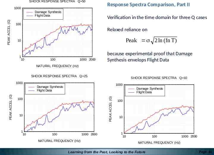
Response Spectra Comparison, Part II NESC ACADEMY WEBCAST SHOCK RESPONSE SPECTRA Q 50 1000 PEAK ACCEL (G) Damage Synthesis Flight Data Verification in the time domain for three Q cases 100 Relaxed reliance on Peak 2 ln (fn T ) 10 1 10 100 1000 2000 because experimental proof that Damage Synthesis envelops Flight Data NATURAL FREQUENCY (Hz) SHOCK RESPONSE SPECTRA Q 25 SHOCK RESPONSE SPECTRA Q 10 1000 1000 Damage Synthesis Flight Data PEAK ACCEL (G) PEAK ACCEL (G) Damage Synthesis Flight Data 100 10 1 10 100 1000 2000 NATURAL FREQUENCY (Hz) 100 10 1 10 100 1000 2000 NATURAL FREQUENCY (Hz) Learning from the Past, Looking to the Future Page: 44
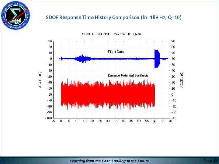
NESC ACADEMY WEBCAST SDOF Response Time History Comparison (fn 189 Hz, Q 10) 30 90 20 80 Flight Data 10 ACCEL (G) fn 189 Hz Q 10 70 0 60 -10 50 -20 40 Damage Potential Synthesis -30 30 -40 20 -50 10 -60 0 -70 -10 -80 -20 -90 -30 -100 -5 0 5 10 15 20 25 30 35 40 45 50 55 Learning from the Past, Looking to the Future 60 65 ACCEL (G) SDOF RESPONSE -40 70 Page: 45
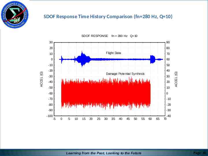
NESC ACADEMY WEBCAST SDOF Response Time History Comparison (fn 280 Hz, Q 10) 30 90 20 80 Flight Data 10 ACCEL (G) fn 280 Hz Q 10 70 0 60 -10 50 -20 40 Damage Potential Synthesis -30 30 -40 20 -50 10 -60 0 -70 -10 -80 -20 -90 -30 -100 -5 0 5 10 15 20 25 30 35 40 45 50 55 Learning from the Past, Looking to the Future 60 65 ACCEL (G) SDOF RESPONSE -40 70 Page: 46
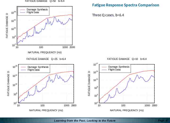
NESC ACADEMY FatigueWEBCAST Response Spectra Comparison FATIGUE DAMAGE Q 50 b 6.4 Damage Synthesis Flight Data FATIGUE DAMAGE D 18 10 Three Q cases, b 6.4 14 10 10 10 6 10 2 10 10 100 1000 2000 NATURAL FREQUENCY (Hz) FATIGUE DAMAGE Q 25 b 6.4 FATIGUE DAMAGE Q 10 b 6.4 17 FATIGUE DAMAGE D 10 10 Damage Synthesis Flight Data FATIGUE DAMAGE D 18 14 10 10 10 6 10 2 10 10 14 10 Damage Synthesis Flight Data 11 10 8 10 5 10 2 100 1000 2000 NATURAL FREQUENCY (Hz) 10 10 100 1000 2000 NATURAL FREQUENCY (Hz) Learning from the Past, Looking to the Future Page: 47
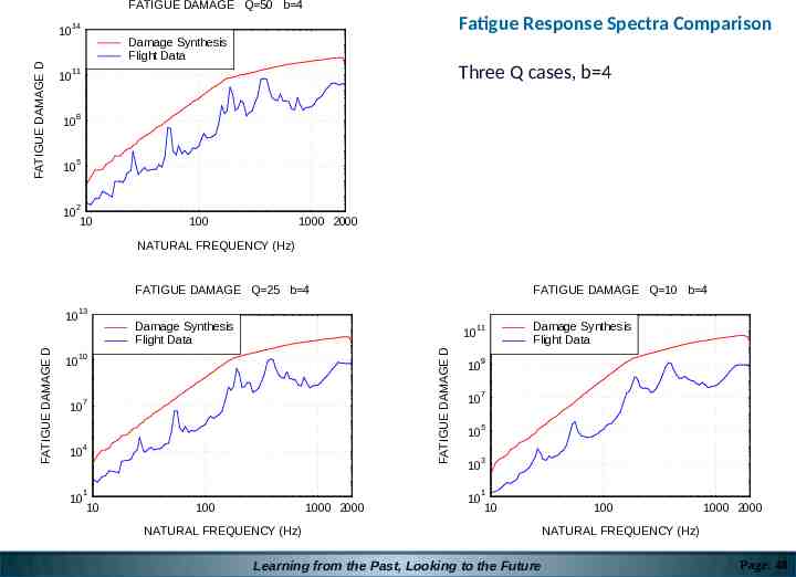
Fatigue Response Spectra Comparison NESC ACADEMY WEBCAST Fatigue Response Spectra Comparison Three Q cases, b 6.4 FATIGUE DAMAGE Q 50 b 4 14 FATIGUE DAMAGE D 10 Damage Synthesis Flight Data Three Q cases, b 4 11 10 8 10 5 10 2 10 10 100 1000 2000 NATURAL FREQUENCY (Hz) FATIGUE DAMAGE Q 25 b 4 FATIGUE DAMAGE Q 10 b 4 13 Damage Synthesis Flight Data 11 10 FATIGUE DAMAGE D FATIGUE DAMAGE D 10 10 10 7 10 4 10 1 10 10 Damage Synthesis Flight Data 9 10 7 10 5 10 3 10 1 100 1000 2000 NATURAL FREQUENCY (Hz) 10 10 100 1000 2000 NATURAL FREQUENCY (Hz) Learning from the Past, Looking to the Future Page: 48
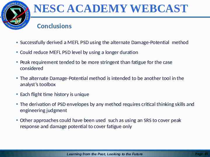
NESC ACADEMY WEBCAST Conclusions Successfully derived a MEFL PSD using the alternate Damage-Potential method Could reduce MEFL PSD level by using a longer duration Peak requirement tended to be more stringent than fatigue for the case considered The alternate Damage-Potential method is intended to be another tool in the analyst’s toolbox Each flight time history is unique The derivation of PSD envelopes by any method requires critical thinking skills and engineering judgment Other approaches could have been used such as using an SRS to cover peak response and damage potential to cover fatigue only Learning from the Past, Looking to the Future Page: 49
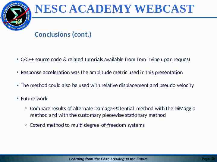
NESC ACADEMY WEBCAST Conclusions (cont.) C/C source code & related tutorials available from Tom Irvine upon request Response acceleration was the amplitude metric used in this presentation The method could also be used with relative displacement and pseudo velocity Future work: o Compare results of alternate Damage-Potential method with the DiMaggio method and with the customary piecewise stationary method o Extend method to multi-degree-of-freedom systems Learning from the Past, Looking to the Future Page: 50
NESC ACADEMY WEBCAST As an industry representative to NESC Load & Dynamics I am here to serve you! Please contact: Tom Irvine Dynamic Concepts, Inc Email: [email protected] Phone: 256-922-9888 x343 Learning from the Past, Looking to the Future Page: 51