Magnetic Resonance Imaging: Physical Principles Richard Watts,


40 Slides765.50 KB
Magnetic Resonance Imaging: Physical Principles Richard Watts, D.Phil. Weill Medical College of Cornell University, New York, USA
Physics of MRI, Lecture 1 Nuclear Magnetic Resonance – Nuclear spins – Spin precession and the Larmor equation – Static B0 – RF excitation – RF detection Fourier Transforms – Continuous Fourier Transform – Discrete Fourier Transform – Fourier properties – k-space representation in MRI Spatial Encoding – – – – 03/26/24 Slice selective excitation Frequency encoding Phase encoding Image reconstruction 2
Bibliography Magnetic Resonance Imaging – Physical Principles and Sequence Design. Haacke, Brown, Thompson, Venkatesan. Wiley 1999. The Fourier Transform and It’s Applications. Bracewell. McGraw-Hill 2000. Medical books – simple, but little mathematical depth Physics books – more depth, but more complicated Web: http://mri.med.cornell.edu/links.html 03/26/24 3
Nuclear Spins Rotating charges correspond to an electrical current Current gives a magnetic moment, Nuclear spin, electron spin and electron orbit Moments align with external magnetic field 03/26/24 P ro to n E le c tro n 4
Spin Precession B Magnetic “Spinning Top” d dt B Bloch equation with no relaxation Gyromagnetic ratio Precession frequency B Larmor equation For protons, 42.58 MHz/T 03/26/24 5
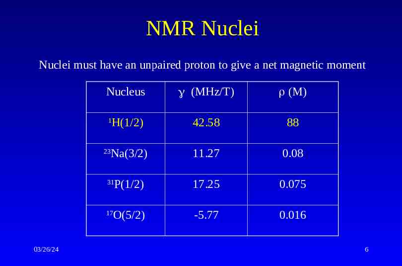
NMR Nuclei Nuclei must have an unpaired proton to give a net magnetic moment Nucleus (MHz/T) (M) H(1/2) 42.58 88 Na(3/2) 11.27 0.08 P(1/2) 17.25 0.075 O(5/2) -5.77 0.016 1 23 31 17 03/26/24 6
B0 Field Higher static field gives greater polarization of the spins at a given temperature more signal B0 0.5T can be achieved using permanent magnets (large, heavy, but cheap to maintain) B0 0.5T requires superconducting magnet (expensive, requires liquid nitrogen and helium cooling). Quenching possible! B0 must be uniform to high accuracy ( 1 in 106) over the volume to be imaged Typical clinical scanner uses 1.5T superconducting magnet. Larmor frequency 64MHz 03/26/24 7
RF Excitation Energy is put into the spins by a small alternating magnetic field, b1, at the resonant frequency of the spin precession ˆ B B0 zˆ b1 cos t x For typical DC field strengths 0.5-7T the resonant frequency is in the radio frequency (RF) part of the electromagnetic spectrum Interference to/from other RF sources can be a problem – requires shielding 03/26/24 8
RF Excitation m 03/26/24 rotating frame 9
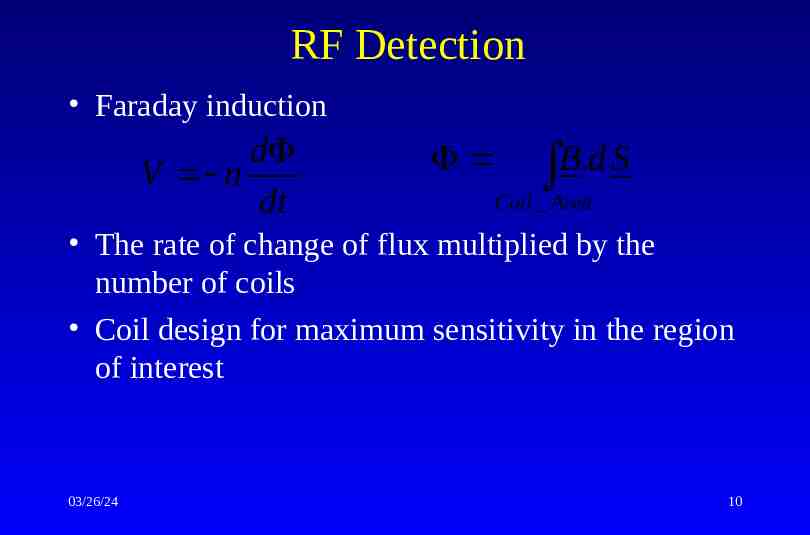
RF Detection Faraday induction d V n dt B.d S Coil Area The rate of change of flux multiplied by the number of coils Coil design for maximum sensitivity in the region of interest 03/26/24 10
Spatial Encoding Three gradient coils allow the magnetic field to vary in any direction (linear combination) B ( B0 Gx x G y y Gz z ) zˆ Spatial information comes from the variation in Larmor frequency due to the field gradient No moving parts to acquire different views/acquisition parameters Gradient coils require switching current rapidly in a high magnetic field vibration noise 03/26/24 11
Slice Selective Excitation Gradient field I B ( B0 Gz z ) zˆ ( B0 Gz z ) 03/26/24 B ( B 0 G z z ) Gradient strength, center frequency and bandwidth of rf pulse determines slice selected B 1 0 C e n te r F re q u e n c y P o s itio n , z 12
Gradient Coils Field always along z Gradient along x, y, or z I B ( B0 Gx x G y y Gz z ) zˆ Usually, only one gradient active at a time, but can combine to give any arbitrary direction 03/26/24 G z I G y I 13
Frequency Encoding Apply magnetic field gradient along x-axis during data read-out B ( B0 Gx x) zˆ ( B0 Gx x) Frequency of signal depends on the x-position of the spins from which it is generated Fourier transform from (spatial) frequency space to image space 03/26/24 14
Phase Encoding Apply magnetic field gradient along y-axis prior to read-out for a time t B ( B0 G y y ) zˆ ( B0 G y y ) 0 . t Phase of spins depends on y-position Repeat acquisition for different phase encoding amplitudes 03/26/24 15
Image Reconstruction Spins from all positions (voxels) contribute signals to each measurement (sample) The frequency and phase of the signal from each voxel is determined by its spatial position How do we form an image? Fourier Transforms! 03/26/24 16
Fourier Transforms 1 Example: Sound What is sound? An oscillating pressure wave in the air. Pressure is a function of time f(t) How do we hear? Our ears contain hair-like structures that resonate at different frequencies. What we detect is the amplitude of each frequency, F(ν) What is the mathematical relation between f(t) and F(ν)? 03/26/24 17
Fourier Transforms 2 To measure the signal at a given frequency, multiply by a sine/cosine wave at that frequency and integrate – all other frequencies 0 F ( ) f (t )e 2 i t dx This is the continuous Fourier transform i Note that e cos i. sin e 03/26/24 i 1 18
Fourier Transforms 3 Time/Frequency (t/ ) domain Position/Spatial Frequency (x, k) domain Fourier Transform 2 i t 2 ikx F ( ) f ( t ) e dt F ( k ) f ( x ) e dx t , x k Inverse Fourier Transform t, k x 03/26/24 f (t ) F ( )e 2 i t d f ( x) F (k )e 2 ikx dk 19
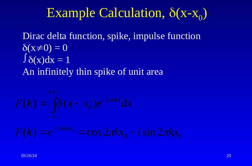
Example Calculation, (x-x0) Dirac delta function, spike, impulse function (x 0) 0 (x)dx 1 An infinitely thin spike of unit area F (k ) ( x x0 )e 2 ikx dx F (k ) e 03/26/24 2 ikx0 cos 2 kx0 i sin 2 kx0 20
Example Calculation, (x-x0) Fourier Transform of a Delta-Function at k 0 Fourier Transform of a Delta-Function at k 4 1 1 Fourier Transform, Real Fourier Transform, Imaginary Delta Function 0 0 0 32 64 96 128 0 32 64 128 Fourier Transform, Real -1 -1 96 x, k x, k Fourier Transform, Imaginary Delta Function Fourier Transform of a Delta-Function at k 8 1 0 0 03/26/24 32 64 96 128 Fourier Transform, Real -1 x, k Fourier Transform, Imaginary Delta Function 21
Example Calculation, Boxcar Boxcar (Rect) function of width a at the origin f(-a/2 x a/2) 1, otherwise f(x) 0 a / 2 F (k ) f ( x)e F (k ) dx cos(2 kx)dx a/2 Note: f(x) is even so F(k) must be real 1 sin(2 kx) aa // 22 1 2 sin(2 ka / 2) 2 k 2 ik F (k ) 03/26/24 2 ikx sin( ka) a sin c( ka) k Useful result relating to the point-spread function for finite sampling - later 22
Example Calculation, Boxcar Fourier Transform of Boxcar 40 Fourier Transform, Real Fourier Transform, Imaginary 30 Boxcar Function 20 10 0 0 32 64 96 128 -10 03/26/24 x, k 23
Discrete Fourier Transform (DFT) Signal in MRI is continuous over all spatial frequencies, but only a set of uniformly spaced measurements are made. Discrete sampling at k p k and x q x (p,q integers). Replace integral with finite summation: F (k ) f ( x)e 03/26/24 2 ikx dx n 1 F ( p k ) f (q x)e q n 2 i ( p k )( q x ) 24
Continuous vs. Discrete Fourier Transform Continuous Fourier Transform Discrete F (k ) f ( x)e 2 ikx dx f ( x) F (k )e 03/26/24 F ( p k ) f (q x)e 2 i ( p k )( q x ) q n Inverse Fourier Transform n 1 2 ikx dk 1 f (q x) 2n n 1 2 ipq / 2 n F ( p k ) e p n 25
Sampling Effects k Spatial frequency step Due to the cyclical nature of the sine wave, e 2 i ( p k )( q x ) e 2 i ( p k )( q x ) .e 2 ip e 2 i ( p k )( q x 1 / k ) Hence, a signal at x x0 cannot be distinguished from one at x x0 1/ k 1/ k Field of view, FOV 03/26/24 p k Highest spatial frequency This determines the resolution of the image obtained The point-spread function can be calculated – intrinsic blurring of the reconstructed image 26
Nyquist Sampling Criterion The sampling field of view, 1/ k must be greater than the object dimension, A ie. 1 k A If this is not fulfilled, wrap-around artifacts are produced 03/26/24 27
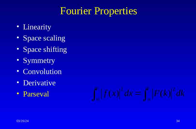
Fourier Properties Linearity Space scaling Space shifting Symmetry Convolution Derivative Parseval 03/26/24 f ( x) g ( x) F (k ) G (k ) 28
Fourier Properties Linearity Space scaling Space shifting Symmetry Convolution Derivative Parseval 03/26/24 1 k f (ax) F a a 29
Fourier Properties Linearity Space scaling Space shifting Symmetry Convolution Derivative Parseval 03/26/24 f ( x a ) F ( k )e 2 ika 30
Fourier Properties Linearity Space scaling Space shifting Symmetry Convolution Derivative Parseval 03/26/24 F(k) f(x) Real Part Imaginary Part Real Even Odd Imaginary Odd Even 31
Fourier Properties Linearity Space scaling Space shifting Symmetry Convolution Derivative Parseval 03/26/24 f ( x) g ( x) F (k )G (k ) 32
Fourier Properties Linearity Space scaling Space shifting Symmetry Convolution Derivative Parseval 03/26/24 f ( x) 2 ikF (k ) 33
Fourier Properties Linearity Space scaling Space shifting Symmetry Convolution Derivative Parseval 03/26/24 2 2 f ( x) dx F (k ) dk 34
k-space Representation in 1D Magnetic field is sum of static and time-varying gradient fields Bz Bz ( z , t ) B0 z.G (t ) ( z , t ) 0 G ( z , t ) G (t ) z G ( z , t ) ( z.G (t )) Demodulate at 0, accumulated phase G G ( z , t ) G ( z , t )dt z G (t )dt 03/26/24 35
Aside - Signal Demodulation Signal measured has a frequency of 64 MHz at 1.5T. We are only interested in frequency or phase changes relative to 0. Signal is demodulated by multiplying by a sine wave at 0 1 sin(a ). sin(b) 2 cos(a b) cos(a b) sin ( 0 )t . sin( 0t ) 1 cos( )t cos( 0t ) 2 Effectively we move into the frame of reference of the center frequency. Analogue band-pass filters get rid of higher frequencies 03/26/24 36
k-space Representation in 1D Signal is the integration of the spin density (z) over z, accounting for phase variations s (t ) ( z )e i dz Define k k(t) as 2 kz k (t ) G (t )dt 2 Hence, 2 ikz s (k ) ( z )e dz The signal measured s(k) is the Fourier transform of the spin density 03/26/24 37
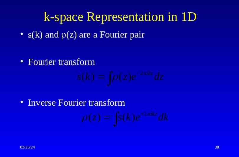
k-space Representation in 1D s(k) and (z) are a Fourier pair Fourier transform s (k ) ( z )e 2 ikz dz Inverse Fourier transform ( z ) s (k )e 03/26/24 2 ikz dk 38
k-space Representation in 3D s(k) s(k), (z) (r) s(k) and (r) are a Fourier pair Fourier transform s (k ) (r )e 2 i k . z dr (r ) s (k )e 2 i k . z dk Inverse Fourier transform Integration is now over a volume 03/26/24 39
k-space and Image-Space Not obvious! 03/26/24 40