The simple Torricelli Mercury Barometer reviewed Chem Factoid: At


27 Slides1.30 MB
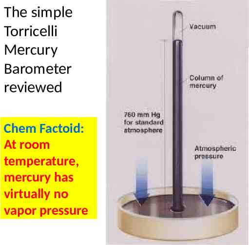
The simple Torricelli Mercury Barometer reviewed Chem Factoid: At room temperature, mercury has virtually no vapor pressure
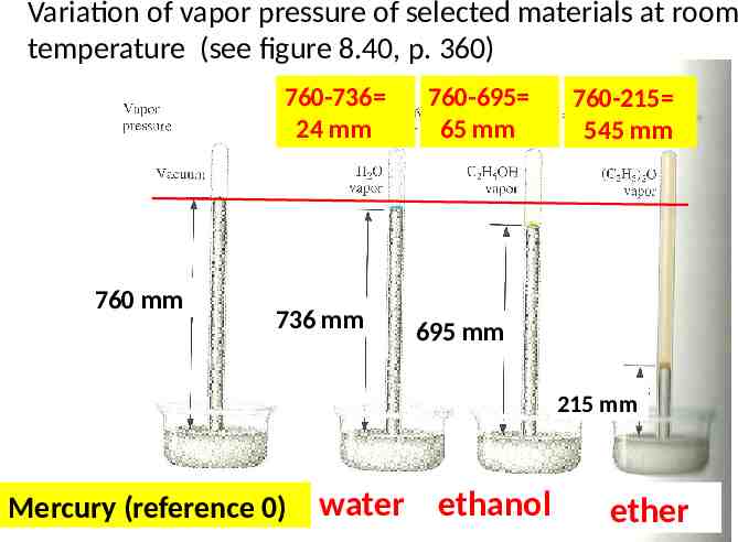
Variation of vapor pressure of selected materials at room temperature (see figure 8.40, p. 360) 760-736 24 mm 760 mm 736 mm 760-695 65 mm 760-215 545 mm 695 mm 215 mm Mercury (reference 0) water ethanol ether
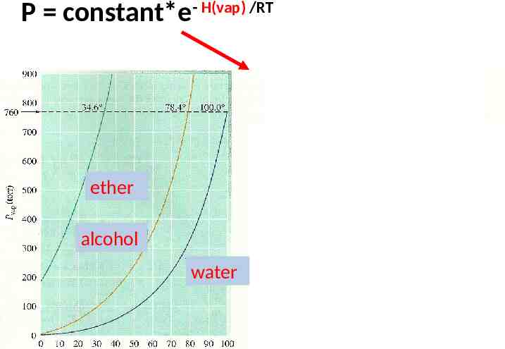
The vapor pressure of materials (duh ) varies with temperature P(mm Hg) vs T 760 mm ether ethanol water Common sense says: the sharper the Ln P(mm Hg) vs T pressure rise, the less strongly the liquid is bound ( e.g. it’s easier ether to escape as a gas) water ethanol
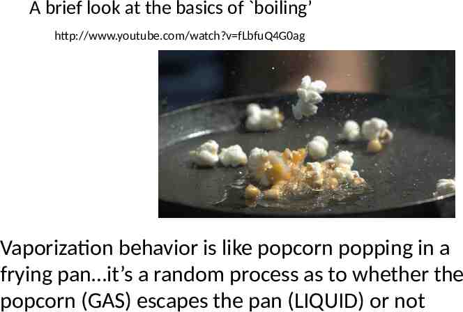
A brief look at the basics of boiling’ http://www.youtube.com/watch?v fLbfuQ4G0ag Vaporization behavior is like popcorn popping in a frying pan it’s a random process as to whether the popcorn (GAS) escapes the pan (LIQUID) or not
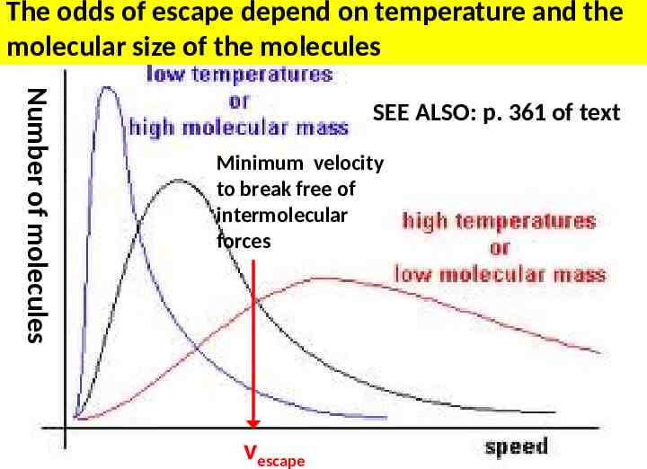
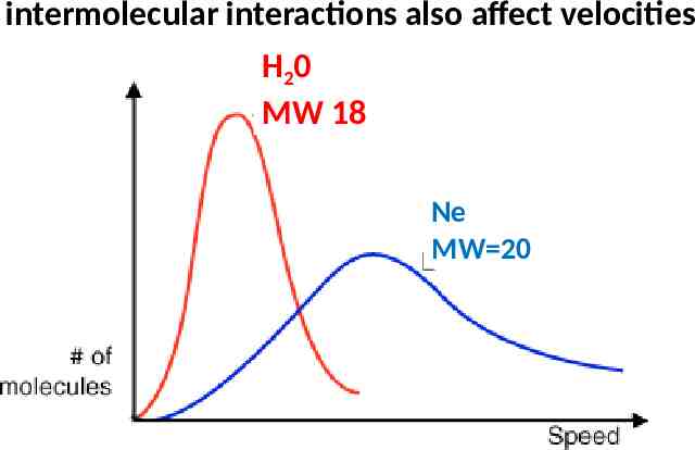
The odds of escape depend on temperature and the molecular size of the molecules Number of molecules SEE ALSO: p. 361 of text Minimum velocity to break free of intermolecular forces vescape
intermolecular interactions also affect velocities H20 MW 18 Ne MW 20
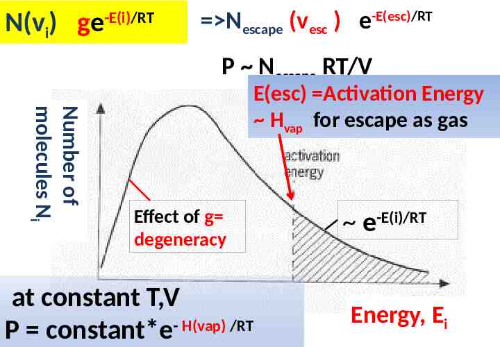
N(vi) ge -E(i)/RT Nescape (vesc ) e-E(esc)/RT P Nescape RT/V Number of molecules Ni E(esc) Activation Energy Hvap for escape as gas Effect of g degeneracy at constant T,V P constant*e- H(vap) /RT e-E(i)/RT Energy, Ei
P constant*e- H(vap) /RT Ln P A - Hvap RT ether alcohol water
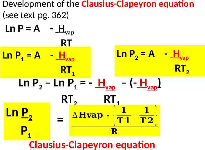
Development of the Clausius-Clapeyron equation (see text pg. 362) Ln P A - Hvap RT Ln P1 A - Hvap RT1 Ln P2 A - Hvap RT2 Ln P2 – Ln P1 - Hvap – (- Hvap) RT2 RT1 Ln P2 P1 𝟏 𝟏 𝐇𝐯𝐚𝐩 𝐓𝟏 𝐓 𝟐 𝐑 { } Clausius-Clapeyron equation
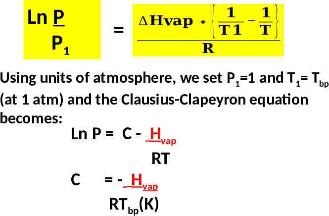
Ln P P1 𝟏 𝟏 𝐇𝐯𝐚𝐩 𝐓𝟏 𝐓 𝐑 { } Using units of atmosphere, we set P1 1 and T1 Tbp (at 1 atm) and the Clausius-Clapeyron equation becomes: Ln P C - Hvap RT C - Hvap RTbp(K)
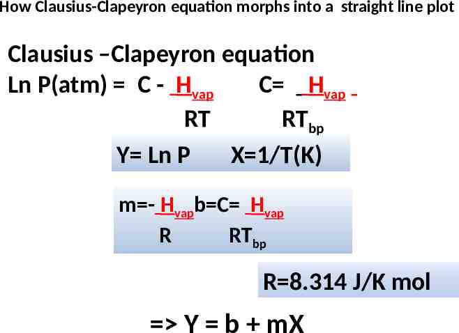
How Clausius-Clapeyron equation morphs into a straight line plot Clausius –Clapeyron equation Ln P(atm) C - Hvap C Hvap RT RTbp Y Ln P X 1/T(K) m - Hvapb C Hvap R RTbp R 8.314 J/K mol Y b mX
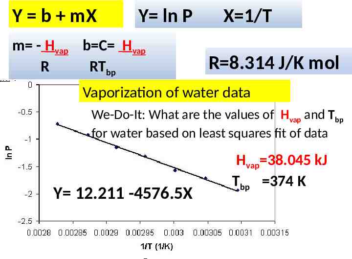
Y b mX Y ln P m - Hvap b C Hvap R RTbp X 1/T R 8.314 J/K mol Vaporization of water data We-Do-It: What are the values of Hvap and Tbp for water based on least squares fit of data Y 12.211 -4576.5X Hvap 38.045 kJ Tbp 374 K
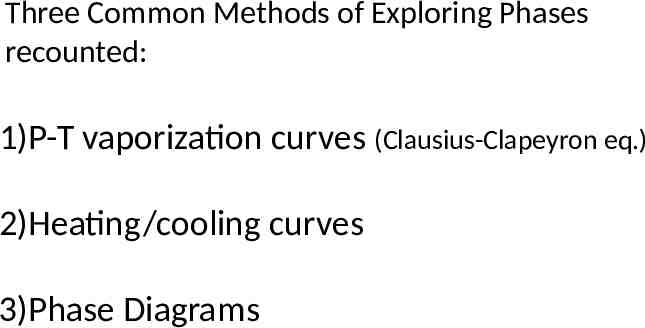
Three Common Methods of Exploring Phases recounted: 1)P-T vaporization curves (Clausius-Clapeyron eq.) 2)Heating/cooling curves 3)Phase Diagrams
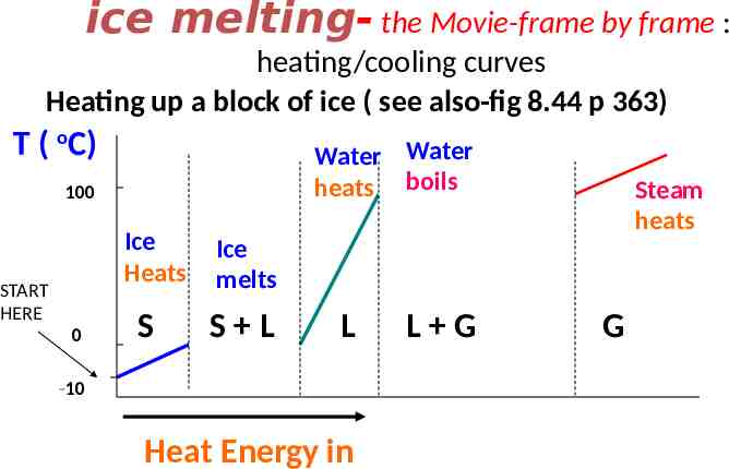
ice melting- the Movie-frame by frame : heating/cooling curves Heating up a block of ice ( see also-fig 8.44 p 363) T ( oC) Water Water heats boils 100 Ice Heats START HERE 0 S Steam heats Ice melts S L L -10 Heat Energy in L G G
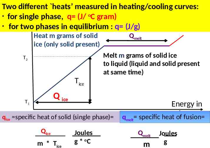
Two different heats’ measured in heating/cooling curves: for single phase, q (J/ oC gram) for two phases in equilibrium : q (J/g) Heat m grams of solid ice (only solid present) Qmelt Melt m grams of solid ice to liquid (liquid and solid present at same time) T2 Tice Q ice T1 qice specific heat of solid (single phase) Qice m * Tice Joules g * oC Energy in qmelt specific heatcal of fusion Qmelt m Joules g
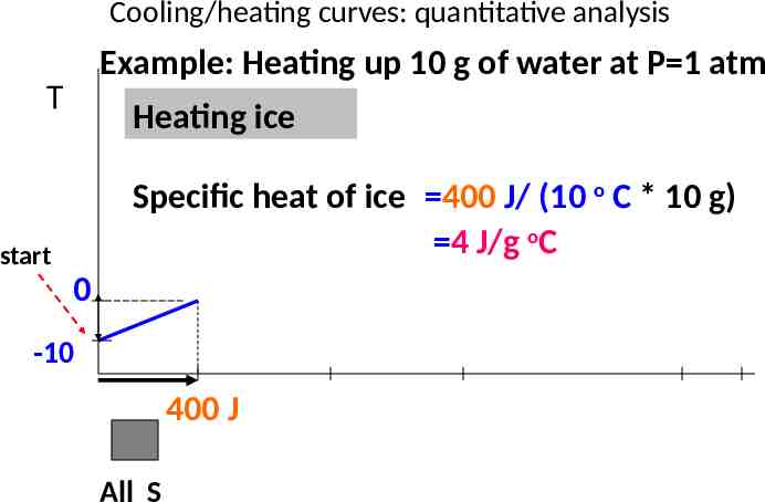
Cooling/heating curves: quantitative analysis Example: Heating up 10 g of water at P 1 atm T Heating ice Specific heat of ice 400 J/ (10 o C * 10 g) 4 J/g oC start 0 -10 400 J All S
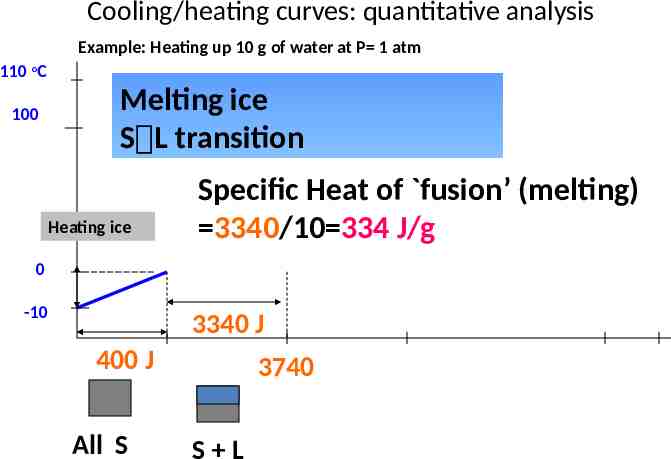
Cooling/heating curves: quantitative analysis Example: Heating up 10 g of water at P 1 atm 110 oC 100 Melting ice S L transition Heating ice Specific Heat of fusion’ (melting) 3340/10 334 J/g 0 -10 3340 J 400 J All S 3740 S L
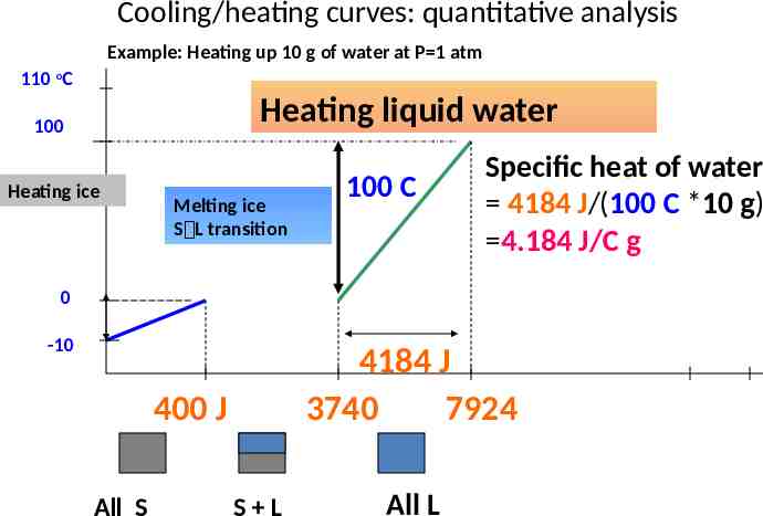
Cooling/heating curves: quantitative analysis Example: Heating up 10 g of water at P 1 atm 110 oC Heating liquid water 100 Heating ice Melting ice S L transition 100 C Specific heat of water 4184 J/(100 C *10 g) 4.184 J/C g 0 -10 4184 J 3740 7924 400 J All S S L All L
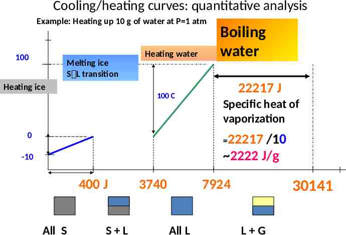
Cooling/heating curves: quantitative analysis Example: Heating up 10 g of water at P 1 atm 100 Melting ice S L transition Heating ice Heating water 100 C 0 Boiling water 22217 J Specific heat of vaporization 22217 /10 2222 J/g -10 400 J All S S L 3740 7924 All L 30141 L G
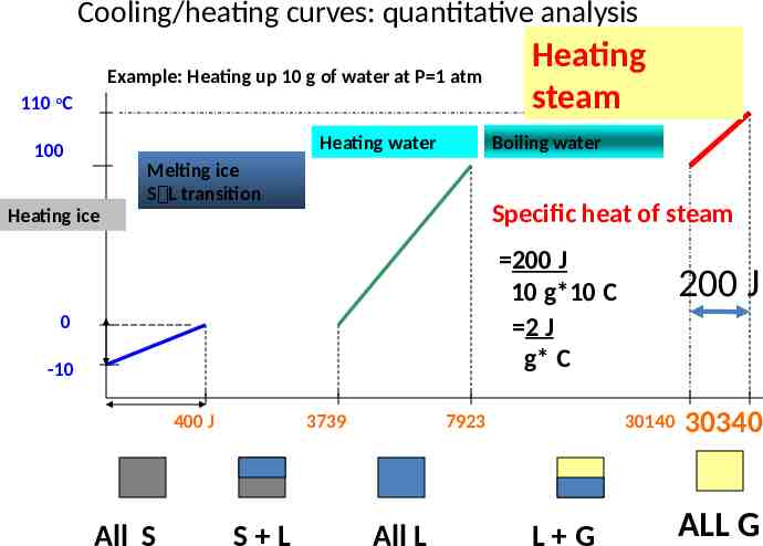
Cooling/heating curves: quantitative analysis Example: Heating up 10 g of water at P 1 atm 110 oC Heating water 100 Heating steam Boiling water Melting ice S L transition Specific heat of steam Heating ice 200 J 10 g*10 C 2 J g* C 0 -10 400 J All S 3739 S L 7923 All L 200 J 30140 L G 30340 ALL G
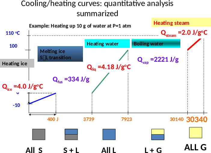
Cooling/heating curves: quantitative analysis summarized Example: Heating up 10 g of water at P 1 atm Heating steam Qsteam 2.0 J/goC 110 oC Heating water 100 Boiling water Melting ice S L transition Heating ice Qice 4.0 J/goC Qliq 4.18 J/goC Qvap 2221 J/g Qfus 334 J/g 0 -10 400 J All S 3739 S L 7923 All L 30140 L G 30340 ALL G
Three Common Methods of Exploring Phases recounted: 1)P-T vaporization curves (Clausius-Clapeyron eq.) 2)Heating/cooling curves 3)Phase Diagrams
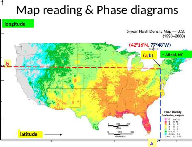
Map reading & Phase diagrams longitude (42 16'N, 77 48‘W) (a,b) b latitude a Alfred, NY
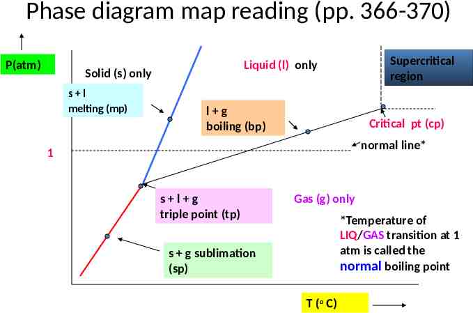
Phase diagram map reading (pp. 366-370) P(atm) Solid (s) only s l melting (mp) Supercritical region Liquid (l) only l g boiling (bp) Critical pt (cp) normal line* 1 s l g triple point (tp) Gas (g) only *Temperature of LIQ/GAS transition at 1 atm is called the normal boiling point s g sublimation (sp) T (o C)
Pressure is often under appreciated as a factor in phase changes Cryophorous demo dramatic visual of phase changes as T, P change
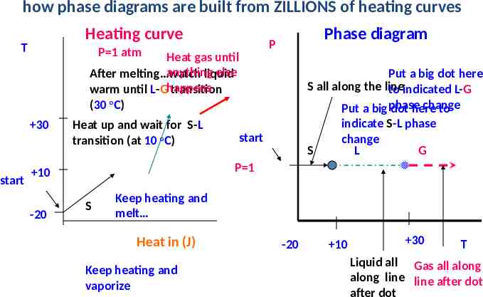
how phase diagrams are built from ZILLIONS of heating curves Heating curve T P 1 atm Heat gas until anything else After melting watch liquid warm until L-Ghappens transition (30 oC) 30 start Heat up and wait for S-L transition (at 10 oC) Put a big dot here S all along the line to indicated L-G change Put a big phase dot here to indicate S-L phase change S L G start P 1 10 -20 Phase diagram P S Keep heating and melt Heat in (J) Keep heating and vaporize -20 10 30 T Liquid all Gas all along along line line after dot after dot
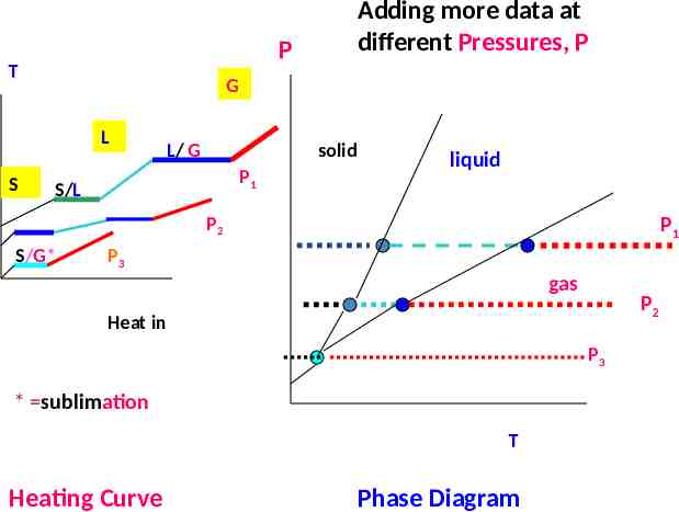
P T G L S Adding more data at different Pressures, P L/ G solid P1 S/L liquid P2 S/G* P1 P3 gas P2 Heat in P3 * sublimation T Heating Curve Phase Diagram