Instructors: Please do not post raw PowerPoint files on public Chapter


23 Slides292.12 KB
Instructors: Please do not post raw PowerPoint files on public Chapter 14 website. Thank you! Using Multiples to Triangulate Results 1
Why Use Multiples? A careful multiples analysis—comparing a company’s multiples versus those of comparable companies—can be useful in improving cash flow forecasts and testing the credibility of DCF-based valuations. Multiples can assist in: 1. Testing the plausibility of forecasted cash flows. 2. Identifying disparities between a company’s performance and those of its competitors. 3. Identifying which companies the market believes are strategically positioned to create more value than other industry players. Multiples analysis is useful only when performed accurately. Poorly performed multiples analysis can lead to misleading conclusions. 2
What Are Multiples? Multiples such as the enterprise-value-to-revenue ratio and the enterprise-value-toEBITA ratio are used to compare the relative valuations of companies. Multiples normalize market values by revenues, profits, asset values, or nonfinancial statistics. Specialty Retail: Trading Multiples, December 2009 million Ticker AZO BBBY BBY HD LOW PETM SHW SPLS Company AutoZone Bed Bath & Beyond Best Buy Home Depot Lowe's Petsmart Sherwin-Williams Staples Market capitalization 7,915 10,368 16,953 49,601 34,814 3,386 7,029 18,054 Debt and debt equivalents 2,783 2,476 11,434 6,060 634 1,099 3,518 Gross enterprise value 10,698 10,368 19,429 61,035 40,874 4,019 8,128 21,572 Net enterprise value 10,535 9,477 18,525 60,510 39,960 3,867 8,044 20,938 Mean Median Deviation (percent)1 1-year forward multiples(times) Revenue 1.5 1.3 0.4 0.9 0.8 0.7 1.1 0.9 EBITDA 7.5 9.5 6.0 9.2 8.3 6.5 9.5 10.1 EBITA 8.5 11.3 7.4 13.0 12.2 10.4 11.4 13.2 1.0 0.9 8.3 8.8 10.9 11.4 38.1% 17.3% 18.2% 1 Deviation Standard deviation/median. 3
Session Overview During this session, we will use three guidelines to build a careful multiples analysis: 1. Use the right multiple. For most analyses, enterprise value to EBITA is the best multiple for comparing valuations across companies. Although the price-toearnings (P/E) ratio is widely used, it is distorted by capital structure and nonoperating gains and losses. 2. Calculate the multiple in a consistent manner. Base the numerator (value) and denominator (earnings) on the same underlying assets. For instance, if you exclude excess cash from value, exclude interest income from the earnings. 3. Use the right peer group. A set of industry peers is a good place to start. Refine the sample to peers that have similar outlooks for long-term growth and return on invested capital (ROIC). 4
Enterprise Value to EBITA When computing and comparing industry multiples, always start with enterprise value to EBITA. It tells more about a company’s value than any other multiple. To see why, consider the key value driver formula developed earlier: Start with the key value driver formula. Substitute EBITA(1 T) for NOPLAT. Divide both sides by EBITA to develop the enterprise value multiple. g NOPLAT 1 ROIC Value WACC g g EBITA(1-T) 1 ROIC Value WACC g g (1 T) 1 Value ROIC EBITA WACC g 5
Enterprise Value to EBITA Let’s use the formula to predict the enterprise-value-to-EBITA multiple for a company with the following financial characteristics: Consider a company growing at 5 percent per year and generating a 15 percent return on invested capital. If the company has an operating tax rate at 30 percent and a 9 percent cost of capital, what multiple of EBITA should it trade at? g (1 T ) 1 Value ROIC EBIT WACC g 5% (1 .30) 1 Value 15% 11.7 EBIT 9% 5% 6
Distribution of EV to EBITA The majority of companies fall between 7 times and 11 times EBITA. If the company or industry you are examining falls outside this range, make sure to identify the reason. S&P 5001: Distribution of Enterprise Value to EBITA, December 2009 Number of observations 1 2 3 4 5 6 7 8 9 10 11 12 13 14 15 16 17 18 19 20 Enterprise value to EBITA 1 Excluding financial institutions, real estate companies, and companies with extremely small or negative EBITA. 7
Why EV to EBITA and Not Price to Earnings? A cross-company multiples analysis should highlight differences in performance, such as differences in ROIC and growth, not differences in capital structure. Although no multiple is completely independent of capital structure, an enterprise value multiple is less susceptible to distortions caused by the company’s debt-to-equity choice. The multiple is calculated as follows: Enterprise Value EBITA MV Debt MV Equity EBITA Consider a company that swaps debt for equity (i.e., raises debt to repurchase equity). EBITA is computed pre-interest, so it remains unchanged as debt is swapped for equity. Swapping debt for equity will keep the numerator unchanged as well. Note, however, that EV may change due to the second-order effects of signaling, increased tax shields, or higher distress costs. 8
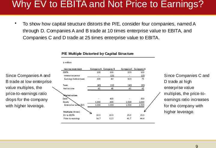
Why EV to EBITA and Not Price to Earnings? To show how capital structure distorts the P/E, consider four companies, named A through D. Companies A and B trade at 10 times enterprise value to EBITA, and Companies C and D trade at 25 times enterprise value to EBITA. P/E Multiple Distorted by Capital Structure million Since Companies A and B trade at low enterprise value multiples, the price-to-earnings ratio drops for the company with higher leverage. Income statement EBITA Interest expense Earnings before taxes Taxes Net income Market values Debt Equity Enterprise value (EV) Multiples (times) EV to EBITA Price to earnings Company A Company B 100 100 (20) 100 80 Company C Company D 100 100 (25) 100 75 (40) 60 (32) 48 (40) 60 (30) 45 1,000 1,000 400 600 1,000 2,500 2,500 500 2,000 2,500 10.0 16.7 10.0 12.5 25.0 41.7 25.0 44.4 Since Companies C and D trade at high enterprise value multiples, the price-toearnings ratio increases for the company with higher leverage. 9
Why EBITA and Not EBITDA? Consider three companies, named A, B, and C. Each company generates the same level of underlying operating profitability; they differ only in size. Since all three companies generate the same level of operating performance, they trade at identical multiples before the acquisition of B by A. Following the acquisition, however, amortization expense causes EBIT to drop for the combined company and the enterprise value-to-EBIT multiple to rise. Enterprise-Value-to-EBIT Multiple Distorted by Acquisition Accounting million Before acquisition EBIT Revenues Cost of sales Depreciation Amortization EBIT Invested capital Organic capital Acquired intangibles Invested capital Enterprise value Multiples (times) EV to EBITA EV to EBIT Company A 375 (150) (75) 150 Company B 125 (50) (25) 50 After A acquires B Company C 500 (200) (100) 200 Company A B 500 (200) (100) (25) 175 Company C 500 (200) (100) 200 750 750 250 250 1,000 1,000 1,000 125 1,125 1,000 1,000 1,125 375 1,500 1,500 1,500 5.0 7.5 5.0 7.5 5.0 7.5 5.0 8.6 5.0 7.5 10
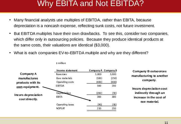
Why EBITA and Not EBITDA? Many financial analysts use multiples of EBITDA, rather than EBITA, because depreciation is a noncash expense, reflecting sunk costs, not future investment. But EBITDA multiples have their own drawbacks. To see this, consider two companies, which differ only in outsourcing policies. Because they produce identical products at the same costs, their valuations are identical ( 3,000). What is each companies EV-to-EBITDA multiple and why are they different? million Company A manufactures products with its own equipment. Incurs depreciation cost directly. Income statement Revenues Raw materials Operating costs EBITDA Depreciation EBITA Operating taxes NOPLAT Company A Company B 1,000 1,000 (100) (250) (400) (400) 500 350 (200) 300 (50) 300 (90) 210 (90) 210 Company B outsources manufacturing to another company. Incurs depreciation cost indirectly through an increase in the cost of raw material. 11
Use Forward-Looking Multiples When building multiples, the denominator should use a forecast of profits, rather than historical profits. – Unlike backward-looking multiples, forward-looking multiples are consistent with the principles of valuation—in particular, that a company’s value equals the present value of future cash flows, not sunk costs. – Second, forward-looking earnings are typically normalized, meaning they better reflect long-term cash flows by avoiding one-time past charges. 12
Use Forward-Looking Multiples To build a forward-looking multiple, choose a forecast year for EBITA that best represents the long-term prospects of the business. In periods of stable growth and profitability, next year’s estimate will suffice. For companies generating extraordinary earnings (either too high or too low) or for companies whose performance is expected to change, use projections further out. Pharmaceuticals: Backward- and Forward-Looking Multiples, December 2007 Price/earnings Enterprise value/EBITA 2007 net income Estimated 2008 EBITA1 Merck 38 Bristol- Myers Squibb Whereas historical P/E ratios across pharmaceutical companies show significant variation Abbott 20 Novartis 20 Pfizer 19 Johnson & Johnson 18 Sanofi-Aventis 16 GlaxoSmithKline 14 Wyeth 13 AstraZeneca 1 2 17 24 Eli Lilly Schering-Plough 16 27 12 N/A2 16 13 Estimated 2012 EBITA1 12 12 12 12 17 13 13 13 15 13 12 the forward-looking EV-to-EBITA multiples are nearly identical. 12 15 12 12 12 15 16 12 11 Consensus analyst forecast. Schering-Plough recorded loss in 2007, so no multiple is reported. 13
Session Overview During this session, we will use three guidelines to build a careful multiples analysis: 1. Use the right multiple. For most analyses, enterprise value to EBITA is the best multiple for comparing valuations across companies. Although the price-toearnings (P/E) ratio is widely used, it is distorted by capital structure and nonoperating gains and losses. 2. Calculate the multiple in a consistent manner. Base the numerator (value) and denominator (earnings) on the same underlying assets. For instance, if you exclude excess cash from value, exclude interest income from the earnings. 3. Use the right peer group. A set of industry peers is a good place to start. Refine the sample to peers that have similar outlooks for long-term growth and return on invested capital (ROIC). 14
Calculate the Multiple in a Consistent Manner There is only one approach to building an enterprise-value-to-EBITA multiple that is theoretically consistent. Enterprise value must include all investor capital but only the portion of value attributable to assets that generate EBITA. Including value in the numerator without including its corresponding income in the denominator will systematically distort the multiple upward. Conversely, failing to recognize a source of investor capital, such as minority interest, will understate the numerator, biasing the multiple downward. If the company holds nonoperating assets or has claims on enterprise value other than debt and equity, these must be accounted for. 15
Consistency: Nonoperating Assets Company A holds only core operating assets and is financed by traditional debt and equity. Company B operates a similar business to Company A, but it also owns 100 million in excess cash and a minority stake in a nonconsolidated subsidiary, valued at 200 million. Since excess cash and nonconsolidated subsidiaries do not contribute to EBITA, they should not be included in the numerator of an EV-to-EBITA multiple. Enterprise Value Multiples and Complex Ownership Company A Company B 100 (18) 82 100 4 (18) 86 Value of core operations Excess cash Nonconsolidated subsidiaries Gross enterprise value 900 900 900 100 200 1,200 Debt Minority interest Market value of equity Gross enterprise value 300 600 900 300 900 1,200 Partial income statement EBITA Interest income Interest expense Earnings before taxes Gross enterprise value 16
Consistency: Include All Financial Claims For Company C, outside investors hold a minority stake in a consolidated subsidiary. Since the minority stake’s value is supported by EBITA, it must be included in the enterprise value calculation. Otherwise, the EV-to-EBITA multiple will be biased downward. The numerator should include not just debt and equity, but also minority interest, the value of unfunded pension liabilities, and the value of employee grants outstanding. Enterprise Value Multiples and Complex Ownership Company A Company C 100 (18) 82 100 (18) 82 Value of core operations Excess cash Nonconsolidated subsidiaries Gross enterprise value 900 900 900 900 Debt Minority interest Market value of equity Gross enterprise value 300 600 900 300 100 500 900 Partial income statement EBITA Interest income Interest expense Earnings before taxes Gross enterprise value 17
Advanced Adjustments For companies with rental expense or pension assets, two additional adjustments can be made. 1. The use of operating leases leads to artificially low enterprise value (missing debt) and EBITA (lease interest is subtracted pre-EBITA). Although operating leases affect both the numerator and denominator in the same direction, each adjustment is of a different magnitude. Enterprise Value Debt PV(Operating Leases) Equity EBITA EBITA Implied Lease Interest 2. To adjust enterprise value for pensions, add the present value of unfunded pension liabilities to debt plus equity. To remove gains and losses related to plan assets, start with EBITA, add back pension expense, and deduct any service costs. Enterprise Value Debt PV(Unfunded Pensions) Equity EBITA EBITA Pension Expense - Service Cost 18
Session Overview During this session, we will use three guidelines to build a careful multiples analysis: 1. Use the right multiple. For most analyses, enterprise value to EBITA is the best multiple for comparing valuations across companies. Although the price-toearnings (P/E) ratio is widely used, it is distorted by capital structure and nonoperating gains and losses. 2. Calculate the multiple in a consistent manner. Base the numerator (value) and denominator (earnings) on the same underlying assets. For instance, if you exclude excess cash from value, exclude interest income from the earnings. 3. Use the right peer group. A set of industry peers is a good place to start. Refine the sample to peers that have similar outlooks for long-term growth and return on invested capital (ROIC). 19
Selecting a Robust Peer Group To create and analyze an appropriate peer group: Start by examining other companies in the target’s industry. But how do you define an industry? Potential resources include the annual report, the company’s Standard Industry Classification (SIC), or its Global Industry Classification (GIC). Once a preliminary screen is conducted, the real digging begins. You must answer a series of strategic questions. Why are the multiples different across the peer group? Do certain companies in the group have superior products, better access to customers, recurring revenues, or economies of scale? 20
Expect Variation Even within an Industry As demonstrated earlier, the enterprise-value-to-EBITA multiple is driven by growth, ROIC, the operating tax rate, and the company’s cost of capital. Be careful comparing across countries. Different tax rates will drive differences in multiples. g (1 T) 1 Value ROIC EBITA WACC g Peers in the same industry will have similar risk profiles and consequently similar costs of capital. Companies with higher ROICs will need less capital to grow. This will drive higher multiples. Since growth will vary across companies, so will their enterprise value multiples. 21
ROIC and Growth Drive Variation The companies below fall into three performance buckets that align with different multiples. The companies with the lowest margins and low growth expectations had multiples of 7 . The companies with low growth but high margins had multiples of 9 . Finally, the companies with high growth and high margins had multiples of 11 to 13 . Factors for Choosing a Peer Group Valuation multiples Enterprise value/ EBITA Company A 7 Company B 7 Company C Company D Company E Company F Consensus projected financial performance Sales growth, 2010–2013 (percent) EBITA margin, 2010 (percent) 5 9 4 9 3 11 13 Low growth, low margin 12 3 6 21 7 8 Performance characteristics 24 Low growth, high margin 24 High growth, high margin 18 22
Closing Thoughts A multiples analysis that is careful and well reasoned not only will provide a useful check of your discounted cash flow (DCF) forecasts but also will provide critical insights into what drives value in a given industry. A few closing thoughts about multiples: 1. Similar to DCF, enterprise value multiples are driven by the key value drivers, return on invested capital and growth. A company with good prospects for profitability and growth should trade at a higher multiple than its peers. 2. A well-designed multiples analysis will focus on operations, will use forecasted profits (versus historical profits), and will concentrate on a peer group with similar prospects. P/E ratios are problematic, as they commingle operating, nonoperating, and financing activities, which leads to misused and misapplied multiples. 3. In limited situations, alternative multiples can provide useful insights. Common alternatives include the price-to-sales ratio, the adjusted price-earnings growth (PEG) ratio, and multiples based on nonfinancial (operational) data. 23