FINANCIAL RISK CHE 5480 Miguel Bagajewicz University of Oklahoma
60 Slides1.74 MB
FINANCIAL RISK CHE 5480 Miguel Bagajewicz University of Oklahoma School of Chemical Engineering and Materials Science 1
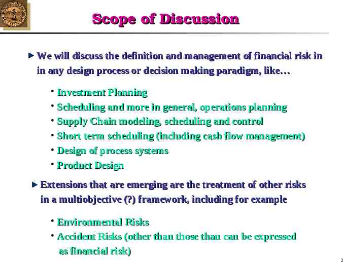
Scope of Discussion We will discuss the definition and management of financial risk in in any design process or decision making paradigm, like Investment Planning Scheduling and more in general, operations planning Supply Chain modeling, scheduling and control Short term scheduling (including cash flow management) Design of process systems Product Design Extensions that are emerging are the treatment of other risks in a multiobjective (?) framework, including for example Environmental Risks Accident Risks (other than those than can be expressed as financial risk) 2
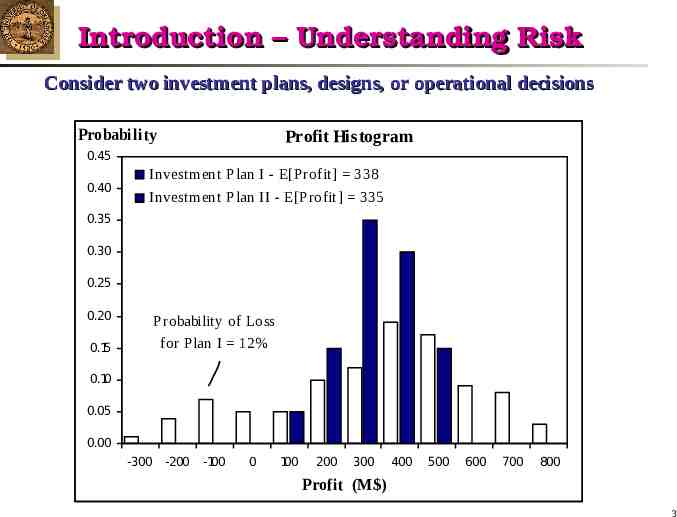
Introduction – Understanding Risk Consider two investment plans, designs, or operational decisions Probability Profit Histogram 0.45 0.40 Investment Plan I - E[P rofit] 338 Investment Plan II - E[Profit ] 335 0.35 0.30 0.25 0.20 0.15 Probability of Loss for Plan I 12% 0.10 0.05 0.00 -300 -200 -100 0 100 200 300 400 500 600 700 800 Profit (M ) 3
Conclusions Risk can only be assessed after a plan has been selected but it cannot be managed during the optimization stage (even when stochastic optimization including uncertainty has been performed). There is a need to develop new models that allow not only assessing but managing financial risk. The decision maker has two simultaneous objectives: Maximize Expected Profit. Minimize Risk Exposure 4
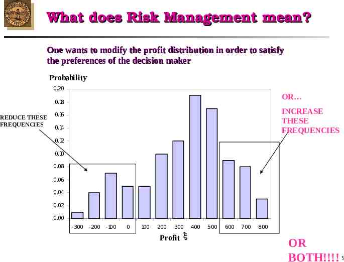
What does Risk Management mean? One wants to modify the profit distribution in order to satisfy the preferences of the decision maker Probability 0.20 OR 0.18 REDUCE THESE FREQUENCIES INCREASE THESE FREQUENCIES 0.16 0.14 0.12 0.10 0.08 0.06 0.04 0.02 0.00 -300 -200 -100 0 100 200 300 Profit x 400 500 600 700 800 OR BOTH!!!! 5
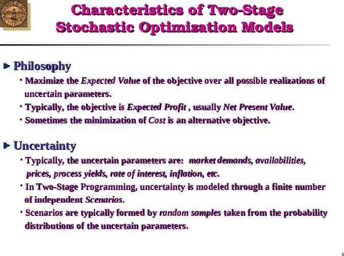
Characteristics of Two-Stage Stochastic Optimization Models Philosophy Maximize the Expected Value of the objective over all possible realizations of uncertain parameters. Typically, the objective is Expected Profit , usually Net Present Value. Sometimes the minimization of Cost is an alternative objective. Uncertainty Typically, the uncertain parameters are: market demands, availabilities, prices, process yields, rate of interest, inflation, etc. In Two-Stage Programming, uncertainty is modeled through a finite number of independent Scenarios. Scenarios are typically formed by random samples taken from the probability distributions of the uncertain parameters. 6
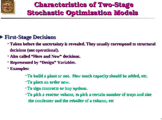
Characteristics of Two-Stage Stochastic Optimization Models First-Stage Decisions Taken before the uncertainty is revealed. They usually correspond to structural decisions (not operational). Also called “Here and Now” decisions. Represented by “Design” Variables. Examples: To build a plant or not. How much capacity should be added, etc. To place an order now. To sign contracts or buy options. To pick a reactor volume, to pick a certain number of trays and size the condenser and the reboiler of a column, etc 7
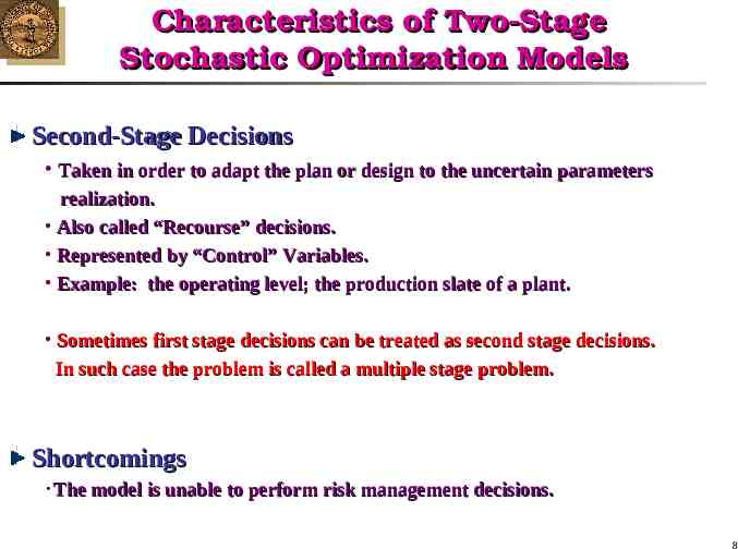
Characteristics of Two-Stage Stochastic Optimization Models Second-Stage Decisions Taken in order to adapt the plan or design to the uncertain parameters realization. Also called “Recourse” decisions. Represented by “Control” Variables. Example: the operating level; the production slate of a plant. Sometimes first stage decisions can be treated as second stage decisions. In such case the problem is called a multiple stage problem. Shortcomings The model is unable to perform risk management decisions. 8
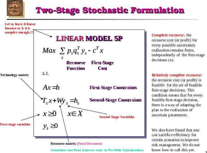
Two-Stage Stochastic Formulation Let us leave it linear because as is it is complex enough.!!! LINEAR MODEL SP Max ps qsT ys cT x s Technology matrix s.t. First-Stage Cost Ax Ax b First-Stage Constraints Ts x Wy s hs Second-Stage Constraints x 0 First stage variables Recourse Function x X Second Stage Variables y s 0 Recourse matrix (Fixed Recourse) Sometimes not fixed (Interest rates in Portfolio Optimization) Complete recourse: the recourse cost (or profit) for every possible uncertainty realization remains finite, independently of the first-stage decisions (x). Relatively complete recourse: the recourse cost (or profit) is feasible for the set of feasible first-stage decisions. This condition means that for every feasible first-stage decision, there is a way of adapting the plan to the realization of uncertain parameters. We also have found that one can sacrifice efficiency for certain scenarios to improve risk management. We do not know how to call this yet. 9
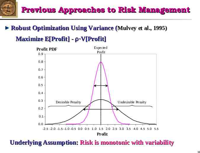
Previous Approaches to Risk Management Robust Optimization Using Variance (Mulvey et al., 1995) Maximize E[Profit] - ·V[Profit] Profit PDF 0.9 Expected Profit 0.8 0.7 0.6 0.5 0.4 0.3 Desirable Penalty Undesirable Penalty Variance is a measure for the dispersion of the distribution 0.2 0.1 0.0 -2.5 -2.0 -1.5 -1.0 -0.5 0.0 0.5 1.0 1.5 2.0 2.5 3.0 3.5 4.0 4.5 5.0 5.5 Profit Underlying Assumption: Risk is monotonic with variability 10
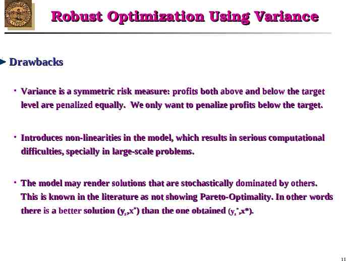
Robust Optimization Using Variance Drawbacks Variance is a symmetric risk measure: profits both above and below the target level are penalized equally. We only want to penalize profits below the target. Introduces non-linearities in the model, which results in serious computational difficulties, specially in large-scale problems. The model may render solutions that are stochastically dominated by others. This is known in the literature as not showing Pareto-Optimality. In other words there is a better solution (ys,x*) than the one obtained (ys*,x*). 11
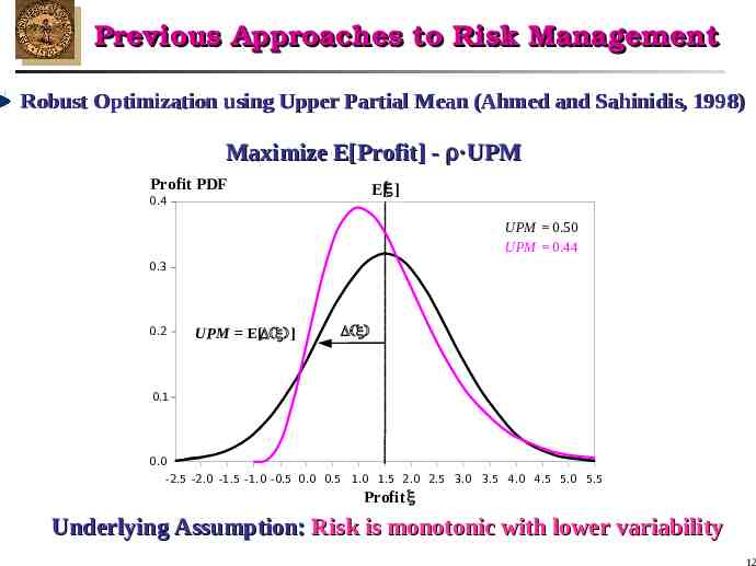
Previous Approaches to Risk Management Robust Optimization using Upper Partial Mean (Ahmed and Sahinidis, 1998) Maximize E[Profit] - ·UPM Profit PDF E[ ] 0.4 UPM 0.50 UPM 0.44 0.3 0.2 UPM E[ ] 0.1 0.0 -2.5 -2.0 -1.5 -1.0 -0.5 0.0 0.5 1.0 1.5 2.0 2.5 3.0 3.5 4.0 4.5 5.0 5.5 Profit Underlying Assumption: Risk is monotonic with lower variability 12
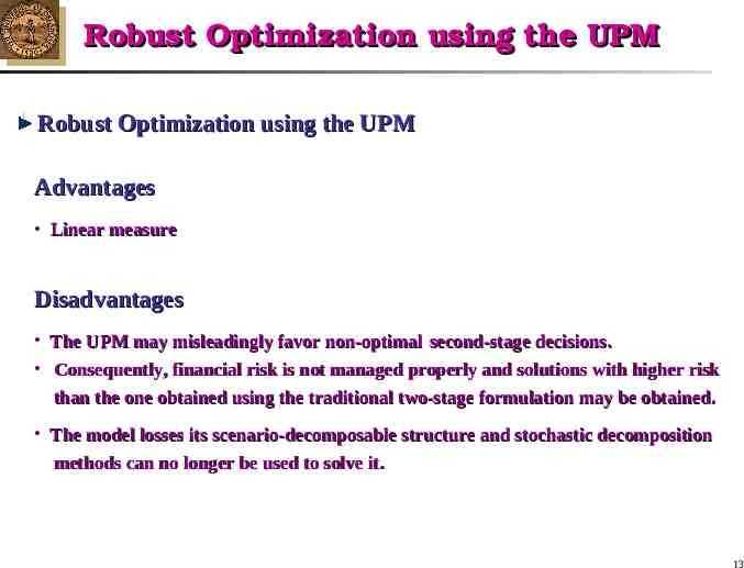
Robust Optimization using the UPM Robust Optimization using the UPM Advantages Linear measure Disadvantages The UPM may misleadingly favor non-optimal second-stage decisions. Consequently, financial risk is not managed properly and solutions with higher risk than the one obtained using the traditional two-stage formulation may be obtained. The model losses its scenario-decomposable structure and stochastic decomposition methods can no longer be used to solve it. 13
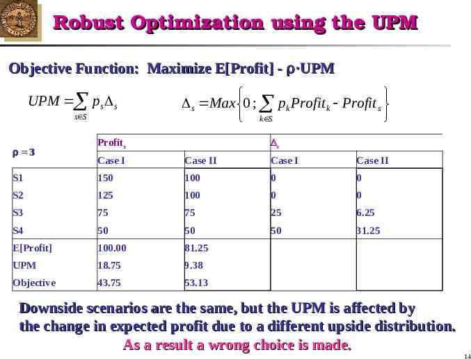
Robust Optimization using the UPM Objective Function: Maximize E[Profit] - ·UPM UPM ps s s S 3 s Max 0 ; pk Profit k Profit s k S Profits s Case I Case II Case I Case II S1 150 100 0 0 S2 125 100 0 0 S3 75 75 25 6.25 S4 50 50 50 31.25 E[Profit] 100.00 81.25 UPM 18.75 9.38 Objective 43.75 53.13 Downside scenarios are the same, but the UPM is affected by the change in expected profit due to a different upside distribution. As a result a wrong choice is made. 14
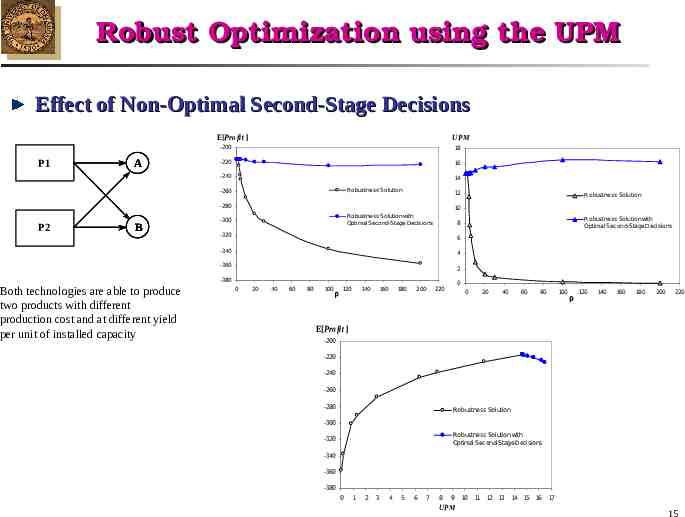
Robust Optimization using the UPM Effect of Non-Optimal Second-Stage Decisions E[Profit ] P1 A UPM -200 18 -220 16 -240 14 R obustness Solution -260 12 -280 P2 B R obustness Solution with Optimal Second-Stage Decisions -300 R obustness Solution with Optimal Second-Stage Decisions 8 -320 6 -340 4 -360 2 -380 Both technologies are able to produce two products with different production cost and at different yield per unit of installed capacity R obustness Solution 10 0 20 40 60 80 100 120 r 140 160 180 200 0 220 0 20 40 60 80 100 r 120 140 160 180 200 220 E[Profit ] -200 -220 -240 -260 -280 R obustness Solution -300 R obustness Solution with Optimal Second-Stage Decisions -320 -340 -360 -380 0 1 2 3 4 5 6 7 8 9 UPM 10 11 12 13 14 15 16 17 15
OTHER APPROACHES Cheng, Cheng, Subrahmanian Subrahmanian and and Westerberg Westerberg (2002, (2002, unpublished) unpublished) Multiobjective Approach: Considers Downside Risk, ENPV and Process Life Cycle as alternative Objectives. Multiperiod Decision process modeled as a Markov decision process with recourse. The problem is sometimes amenable to be reformulated as a sequence of single-period sub-problems, each being a two-stage stochastic program with recourse. These can often be solved backwards in time to obtain Pareto Optimal solutions. This paper proposes a new design paradigm of which risk is just one component. We will revisit this issue later in the talk. 16
OTHER APPROACHES Risk Premium (Applequist, Pekny and Reklaitis, 2000) Observation: Rate of return varies linearly with variability. The of such dependance is called Risk Premium. They suggest to benchmark new investments against the historical risk premium by using a two objective (risk premium and profit) problem. The technique relies on using variance as a measure of variability. 17
Previous Approaches to Risk Management Conclusions The minimization of Variance penalizes both sides of the mean. The Robust Optimization Approach using Variance or UPM is not suitable for risk management. The Risk Premium Approach (Applequist et al.) has the same problems as the penalization of variance. THUS, Risk should be properly defined and directly incorporated in the models to manage it. The multiobjective Markov decision process (Applequist et al, 2000) is very closely related to ours and can be considered complementary. In fact (Westerberg dixit) it can be extended to match ours in the definition of risk and its multilevel parametrization. 18
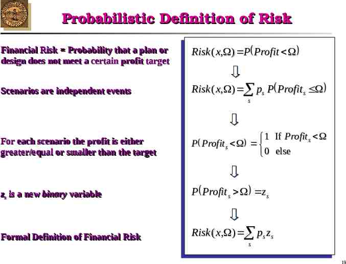
Probabilistic Definition of Risk Financial Financial Risk Risk Probability Probability that that aa plan plan or or design design does does not not meet a certain profit target Risk ( x, ) P Profit Scenarios Scenarios are are independent independent events events Risk ( x, ) ps P Profit s s For For each each scenario scenario the the profit profit is is either either greater/equal greater/equal or or smaller smaller than than the the target target 1 If Profit s P Profit s 0 else zzss is a new binary binary variable P Profit s zs Formal Definition of Financial Risk Risk ( x, ) ps zs s 19
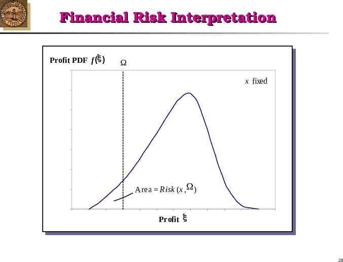
Financial Risk Interpretation Probability Profit PDF f (x ) 0.20 0.14 W W x fixed 0.18 0.12 0.16 0.1 0.10 4 Cumulative Probability Risk (x ,W ) 0.12 0.08 0.10 0.06 0.08 0.06 0.04 0.04 0.02 0.02 Area Risk (x ,W ) 0.00 Profit Profitx x 20
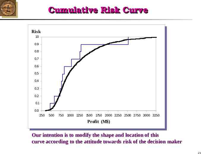
Cumulative Risk Curve Risk 1.0 0.9 0.8 0.7 0.6 0.5 0.4 0.3 0.2 0.1 0.0 250 500 750 1000 1250 1500 1750 2000 2250 2500 2750 3000 3250 Profit (M ) Our intention is to modify the shape and location of this curve according to the attitude towards risk of the decision maker 21
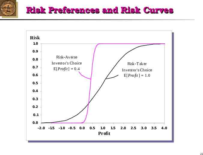
Risk Preferences and Risk Curves Risk 1.0 0.9 0.8 0.7 Risk-Averse Investor's Choice E[Profit ] 0.4 Risk-T aker Investor's Choice E[Profit ] 1.0 0.6 0.5 0.4 0.3 0.2 0.1 0.0 -2.0 -1.5 -1.0 -0.5 0.0 0.5 1.0 1.5 2.0 2.5 3.0 3.5 4.0 Profit 22
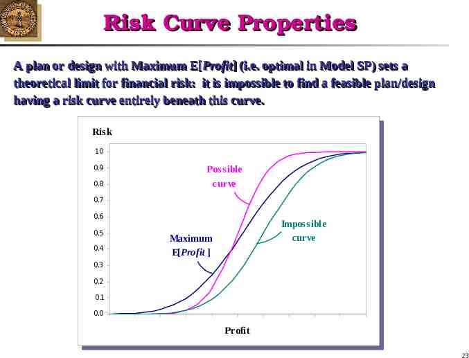
Risk Curve Properties A A plan plan or or design design with with Maximum Maximum E[ E[Profit Profit]] (i.e. (i.e. optimal optimal in in Model Model SP) SP) sets sets a theoretical theoretical limit for financial risk: it is impossible impossible to to find find aa feasible feasible plan/design plan/design having having aa risk risk curve curve entirely entirely beneath beneath this this curve. curve. Risk 1.0 0.9 0.8 Possible curve 0.7 0.6 0.5 0.4 Impossible curve Maximum E[Profit ] 0.3 0.2 0.1 0.0 Profit 23
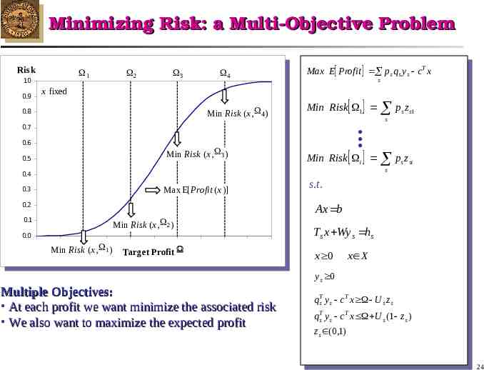
Minimizing Risk: a Multi-Objective Problem Risk W1 1.0 0.9 W2 W3 W4 Max E Profit ps qs y s cT x s x fixed Min Risk (x ,W4) 0.8 Min Risk 1 ps zs1 . . 0.7 0.6 Min Risk (x ,W3 ) 0.5 s Min Risk i ps z si s 0.4 Max E[Profit (x )] 0.3 0.2 s.t. Ax b 0.1 Min Risk (x ,W2 ) 0.0 Min Risk (x ,W1 ) Target Profit W Ts x Wy s hs x 0 x X y s 0 Multiple Objectives: At each profit we want minimize the associated risk We also want to maximize the expected profit qsT y s cT x U s z s qsT y s cT x U s (1 z s ) z s (0,1) 24
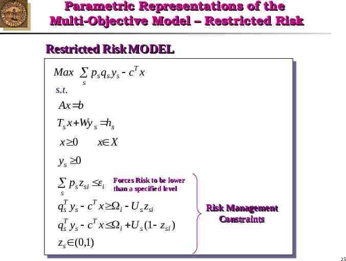
Parametric Representations of the Multi-Objective Model – Restricted Risk Restricted Risk MODEL Max ps qs y s cT x s.t. s Ax b Ts x Wy s hs x 0 x X ys 0 ps z si εi s Forces Risk to be lower than a specified level qsT ys cT x i U s z si qsT ys cT x i U s (1 z si ) Risk Management Constraints Constraints z s (0,1) 25
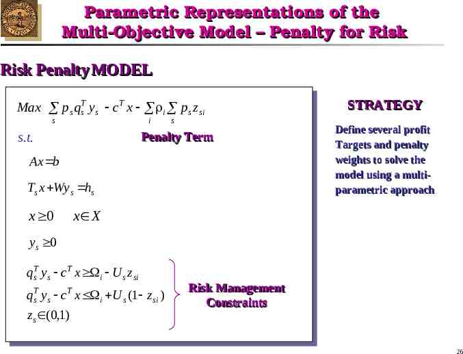
Parametric Representations of the Multi-Objective Model – Penalty for Risk Risk Penalty MODEL Max ps qsT ys cT x i ps z si s i s Penalty Term s.t. Ax b Ts x Wy s hs x 0 STRATEGY Define several profit Targets and penalty weights to solve the model using a multiparametric approach x X y s 0 qsT ys cT x i U s z si qsT ys cT x i U s (1 z si ) z s (0,1) Risk Risk Management Management Constraints Constraints 26
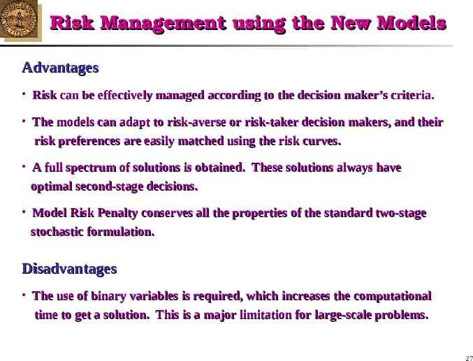
Risk Management using the New Models Advantages Risk can be effectively managed according to the decision maker’s criteria. The models can adapt to risk-averse or risk-taker decision makers, and their risk preferences are easily matched using the risk curves. A full spectrum of solutions is obtained. These solutions always have optimal second-stage decisions. Model Risk Penalty conserves all the properties of the standard two-stage stochastic formulation. Disadvantages The use of binary variables is required, which increases the computational time to get a solution. This is a major limitation for large-scale problems. 27
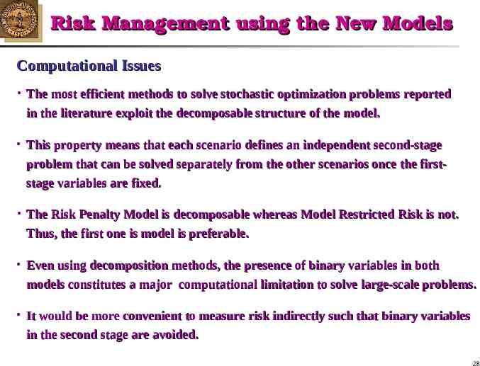
Risk Management using the New Models Computational Issues The most efficient methods to solve stochastic optimization problems reported in the literature exploit the decomposable structure of the model. This property means that each scenario defines an independent second-stage problem that can be solved separately from the other scenarios once the firststage variables are fixed. The Risk Penalty Model is decomposable whereas Model Restricted Risk is not. Thus, the first one is model is preferable. Even using decomposition methods, the presence of binary variables in both models constitutes a major computational limitation to solve large-scale problems. It would be more convenient to measure risk indirectly such that binary variables in the second stage are avoided. 28
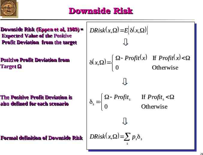
Downside Risk Downside Risk (Eppen (Eppen et et al, al, 1989) 1989) Expected Expected Value Value of of the the Positive Positive Profit Profit Deviation Deviation from from the the target target DRisk x, E x, Positive Profit Deviation from Target Profit x If Profit x x, Otherwise 0 The Positive Profit Deviation is also defined for each scenario Profit s s 0 Formal Formal definition definition of of Downside Downside Risk Risk DRisk x, ps s If Profit s Otherwise s 29
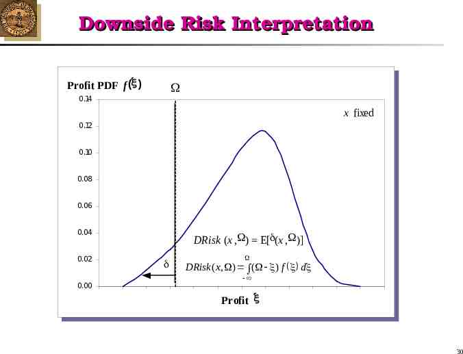
Downside Risk Interpretation Profit PDF f (x ) W 0.14 x fixed 0.12 0.10 0.08 0.06 0.04 0.02 0.00 DRisk (x ,W) E[d(x ,W)] d W DRisk ( x, W) ò(W - x) f ( x ) dx - Profit x 30
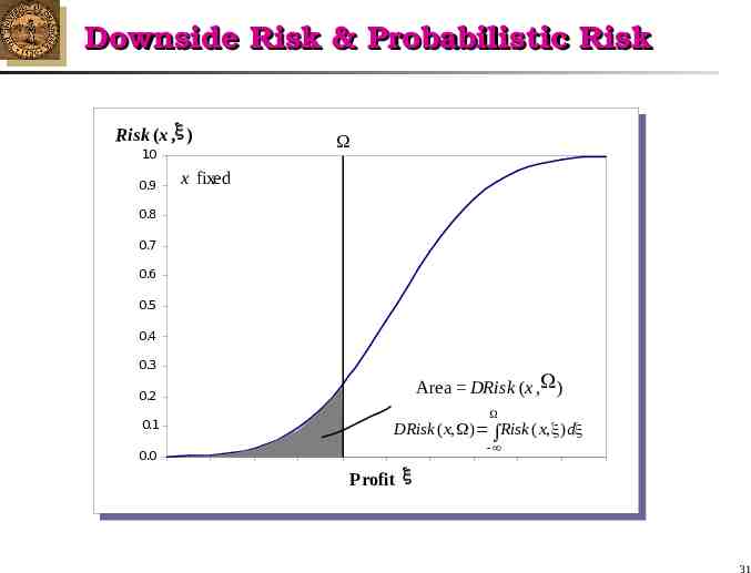
Downside Risk & Probabilistic Risk Risk (x , ) 1.0 0.9 x fixed 0.8 0.7 0.6 0.5 0.4 0.3 Area DRisk (x , ) 0.2 0.1 DRisk ( x, ) Risk ( x, ) d 0.0 Profit 31
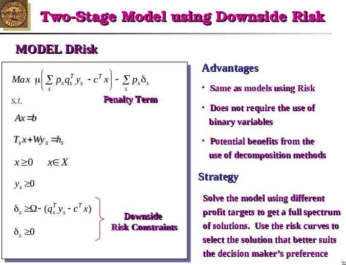
Two-Stage Model using Downside Risk MODEL DRisk Max ps qsT ys cT x ps s s s Penalty Term s.t. Ax b Ts x Wy s hs x 0 s 0 Same as models using Risk Does not require the use of binary variables Potential benefits from the use of decomposition methods x X Strategy y s 0 s Advantages (qsT T ys c x) Downside Downside Risk Constraints Solve the model using different profit targets to get a full spectrum of solutions. Use the risk curves to select the solution that better suits the decision maker’s preference 32
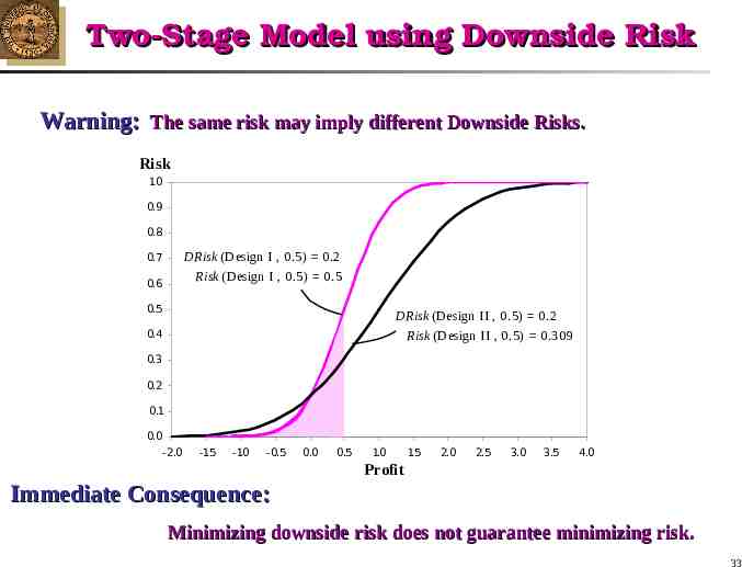
Two-Stage Model using Downside Risk Warning: The same risk may imply different Downside Risks. Risk 1.0 0.9 0.8 DRisk (Design I , 0.5) 0.2 Risk (Design I , 0.5) 0.5 0.7 0.6 0.5 DRisk (Design II , 0.5) 0.2 Risk (Design II , 0.5) 0.309 0.4 0.3 0.2 0.1 0.0 -2.0 -1.5 -1.0 -0.5 0.0 0.5 1.0 1.5 2.0 2.5 3.0 3.5 4.0 Profit Immediate Consequence: Minimizing downside risk does not guarantee minimizing risk. 33
Commercial Software Riskoptimizer (Palisades) and CrystalBall (Decisioneering) Use excell models Allow uncertainty in a form of distribution Perform Montecarlo Simulations or use genetic algorithms to optimize (Maximize ENPV, Minimize Variance, etc.) Financial Software. Large variety Some use the concept of downside risk In most of these software, Risk is mentioned but not manipulated directly. 34
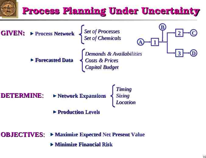
Process Planning Under Uncertainty GIVEN: Process Network Forecasted Data DETERMINE: Set of Processes Set of Chemicals B A Demands & Availabilities Costs & Prices Capital Budget Network Expansions 2 C 3 D 1 Timing Sizing Location Production Levels OBJECTIVES: Maximize Expected Net Present Value Minimize Financial Risk 35
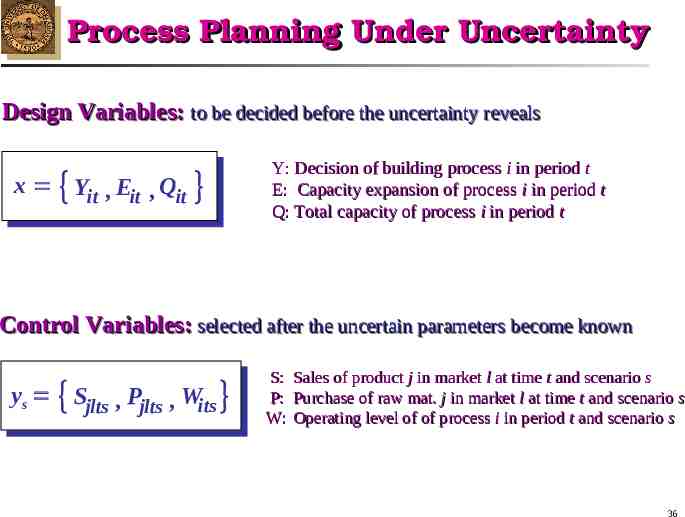
Process Planning Under Uncertainty Design Variables: to be decided before the uncertainty reveals x Yit , Eit , Qit Y: Decision of building process i in period t E: Capacity expansion of process i in period t Q: Total capacity of process i in period t Control Variables: selected after the uncertain parameters become known ys Sjlts , Pjlts , Wits S: Sales of product j in market l at time t and scenario s P: Purchase of raw mat. j in market l at time t and scenario s W: Operating level of of process i in period t and scenario s 36
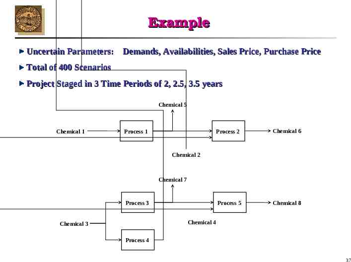
Example Uncertain Parameters: Demands, Availabilities, Sales Price, Purchase Price Total of 400 Scenarios Project Staged in 3 Time Periods of 2, 2.5, 3.5 years Chemical 5 Chemical 1 Process 1 Process 2 Chemical 6 Process 5 Chemical 8 Chemical 2 Chemical 7 Process 3 Chemical 4 Chemical 3 Process 4 37
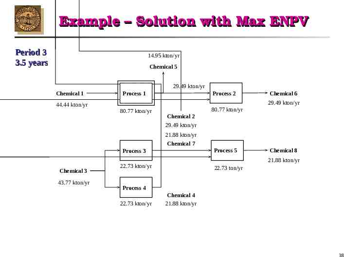
Example – Solution with Max ENPV Period 321 2 years 2.5 3.5 years 14.95 kton/yr Chemical 5 55 Chemical Chemical 5.27 4.71 kton/yr kton/yr 29.49 kton/yr Chemical Chemical 11 44.44 kton/yr 5.27 4.71 kton/yr kton/yr 19.60 41.75 kton/yr 43.77kton/yr kton/yr Chemical 6 29.49 kton/yr 10.23 kton/yr 10.23 80.77 kton/yr Process Process 33 Chemical Chemical333 Chemical Process 2 Process111 Process Process 80.77 kton/yr Chemical 2 29.49 kton/yr Chemical 7 21.88kton/yr kton/yr 20.87 19.60 Chemical7kton/yr 7 Chemical 22.73 22.73 kton/yr kton/yr Process 5 22.73 22.73 kton/yr ton/yr Chemical 8 21.88 20.87 kton/yr kton/yr Process 4 22.73 kton/yr Chemical Chemical44 21.88 20.87kton/yr kton/yr 38
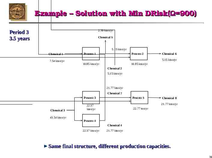
Example – Solution with Min DRisk( 900) 2.39 kton/yr Period 321 2 years 2.5 3.5 years Chemical 5 5.15 kton/yr Chemical 1 7.54 kton/yr Chemical 1 4.99 kton/yr Process 1 10.85 kton/yr Process 1 Chemical 1 10.85 kton/yr 5.59 kton/yr Chemical 5 Chemical 3 Chemical 3 41.70 43.54kton/yr kton/yr Chemical 3 Process Process 44 19.30 kton/yr 22.37 22.37 kton/yr kton/yr Chemical 6 5.15 kton/yr Chemical 5 4.99 kton/yr 10.85 kton/yr Chemical 2 5.59 kton/yr 5.15 kton/yr Process 1 10.85 kton/yr 21.77 kton/yr 20.85 kton/yr7 Chemical Process 3 Process 3 22.37 kton/yr 22.37 kton/yr Process 2 Chemical 7 Process 3 Chemical 7 Process 5 Process 19.305 kton/yr 22.77kton/yr ton/yr 22.43 Chemical 8 Chemical 8 21.77 kton/yr 20.85 kton/yr 22.37 kton/yr Chemical44 Chemical 20.85 kton/yr 21.77 kton/yr Same final structure, different production capacities. 39
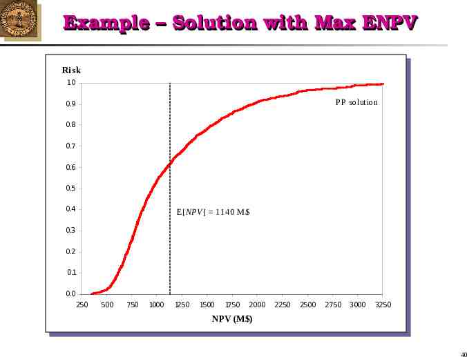
Example – Solution with Max ENPV Risk 1.0 PP solution 0.9 0.8 0.7 0.6 0.5 0.4 E[NPV ] 1140 M 0.3 0.2 0.1 0.0 250 500 750 1000 1250 1500 1750 2000 2250 2500 2750 3000 3250 NPV (M ) 40
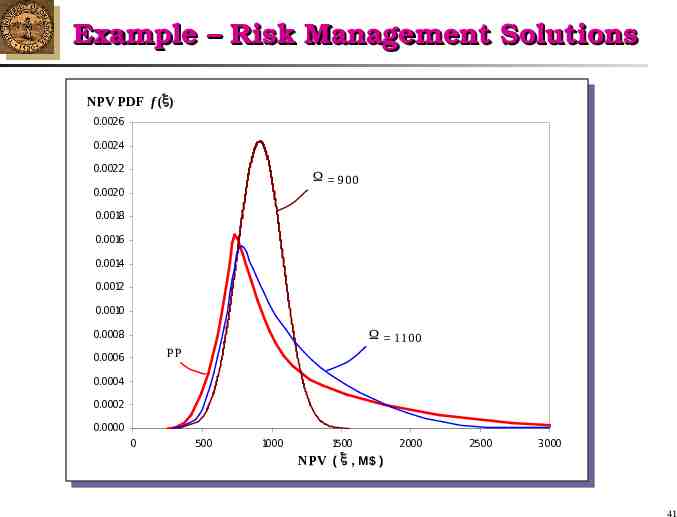
Example – Risk Management Solutions NPV Risk Risk PDF f (x) 1.0 0.0026 0.0024 0.9 0.0022 0.8 0.0020 W 900 W 900 ENPV 908 W 1100 ENPV 1074 W increases 0.7 0.0018 PP ENPV 1140 W PP 0.0016 0.6 500 0.0014 0.5 0.0012 600 0.4 0.0010 900 700 800 1000 0.3 0.0008 0.0006 0.2 W 1100 PP 1200 1300 0.0004 0.1 0.0002 0.0 0.0000 250 0 500 1100 1400 1500 750500 1000 1250 1000 1500 1750 1500 2000 2250 2000 2500 2750 2500 3000 3250 3000 x , M ) NPV NPV ((M ) 41
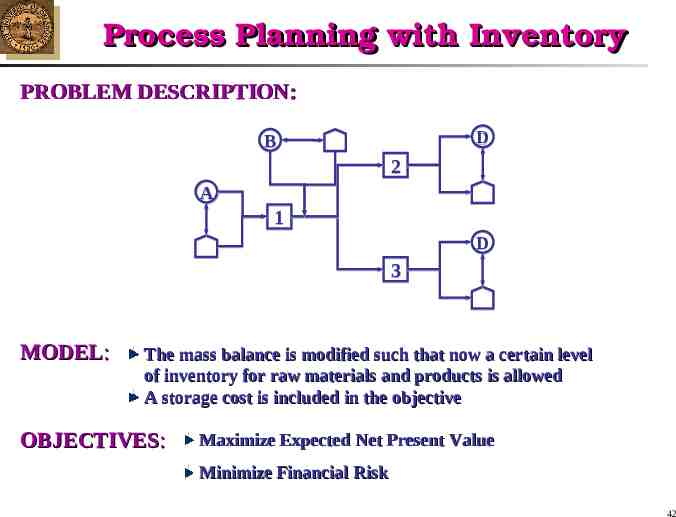
Process Planning with Inventory PROBLEM DESCRIPTION: D B 2 A 1 D 3 MODEL: The mass balance is modified such that now a certain level of inventory for raw materials and products is allowed A storage cost is included in the objective OBJECTIVES: Maximize Expected Net Present Value Minimize Financial Risk 42
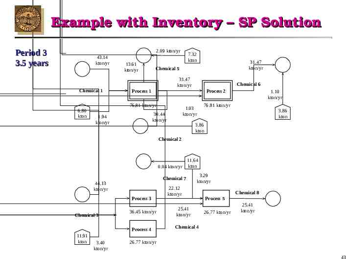
Example with Inventory – SP Solution Period 321 2 years 2.5 3.5 years 33.90 43.14 kton/yr kton/yr 39.04 kton/yr 2.88 kton/yr Chemical 0.42 1 kton/yr Chemical 1 6.80 kton 5.75 kton Chemical 1 1.94 kton/yr 2.09 1.18kton/yr kton/yr 16.28 13.61 11.80 kton/yr kton/yr kton/yr Chemical 5 Chemical55 Chemical Process 11 Process Process 1 51.95 kton/yr 76.81 kton/yr 51.95 kton/yr 12.48 30.44 kton/yr kton/yr 27.24 kton/yr 7.32 10.28 kton kton 5.14 kton/yr 12.48 31.47 kton/yr kton/yr 27.24 kton/yr Process 22 Process Process 2 22.36 kton/yr 76.81 kton/yr 1.03 kton/yr 76.81 kton/yr 1.05 kton/yr 3.86 0.60 kton kton/yr 2.11 Chemical 22 kton Chemical 11.67 kton/yr 26.34 31.47 kton/yr kton/yr Chemical 6 Chemical 6 1.10 Chemical 6kton/yr 0.81 kton/yr 0.90 kton/yr 3.86 kton 1.62 kton Chemical 2 0.04 kton/yr 44.13 kton/yr 35.74 kton/yr 3 ChemicalChemical 3 4.77 kton/yr 11.91 kton 3.40 kton/yr 31.09 kton/yr Process 3 Process 3 36.45 kton/yr 36.45 kton/yr Process 4 11.64 kton Chemical 7 Chemical 7 22.12 kton/yr 3.29 4.65 kton/yr kton/yr 25.41 kton/yr Chemical 8 Process 5 26.77 kton/yr 25.41 kton/yr Chemical 4 26.77 kton/yr 43
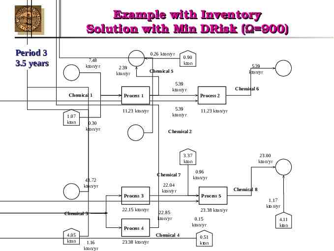
Example with Inventory Solution with Min DRisk ( 900) Period 321 2 years 2.5 3.5 years 0.26 kton/yr 7.48 kton/yr 5.73 kton/yr Chemical 1 0.02 kton/yr 2.39 kton/yr 6.63 5.61 kton/yr kton/yr Process 1 0.90 kton 0.64 Chemical 5 kton 5.80 Chemical0.10 5 5.39 Chemical 5 kton/yr kton/yr kton/yr Process 2 0.51 Process 1 5.39 11.23 kton/yr kton/yr Process 1 kton/yr 1.07 Chemical 1 kton Chemical 1 11.23 kton/yr 0.30 1.01 kton/yr 11.23 kton/yr Chemical 2 kton 41.68 kton/yr 43.72 kton/yr Chemical 3 Chemical 3 7.27 kton 1.29 4.05 kton/yr kton 1.16 kton/yr 5.39 kton/yr 0.32 kton/yr Chemical 6 11.23 kton/yr 20.54 7.38 kton/yr kton 23.00 3.37 1.60 kton/yr Chemicalkton 7 kton/yr 18.46 3.69 Chemical 0.96 7 kton/yr kton/yr 20.58 Chemical 7 kton/yr kton/yr 25.79 3 Process 5 Process Chemical 8 22.04 kton/yr Chemical 8 kton/yr Process 3 22.18 Process 5 Process 22.153kton/yr 23.38 kton/yr 1.17 kton/yr Chemical 3 kton/yr 22.15 kton/yr 22.15 kton/yr Chemical 423.38 kton/yr 22.85 1.64 3.64 Process 4 kton/yr 0.15 4.11 kton/yr kton/yr kton/yr kton Process 23.384kton/yr Chemical0.20 4 kton/yr 0.51 23.38 kton/yr kton 44
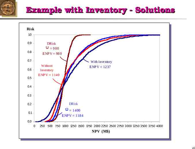
Example with Inventory - Solutions Risk Risk 1.0 1 .0 0.9 DRisk 0.8 0.8 900 PP solution ENPV 980 E[NPV ] 1140 M W 0.7 PPI solution E[NPV ] 1237 M WithPPI Inventory Without PPI Inventory 0.6 0.6 ENPV 1237 ENPV 1140 0.5 0.4 0.3 DRisk 0.2 W 1400 0.1 ENPV 1184 0.0 0 250 500 750 1000 1250 1500 1750 2000 2250 2500 2750 3000 3250 3500 3750 4000 NPV NPV (M ) (M ) 45
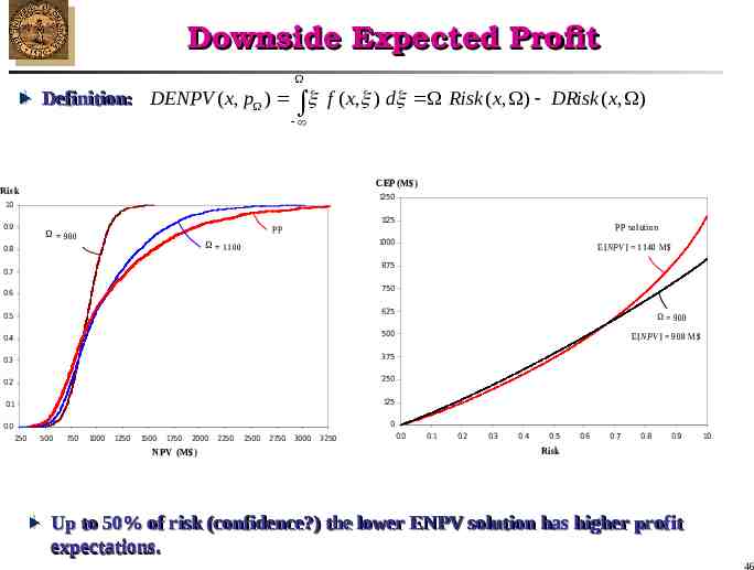
Downside Expected Profit Definition: Definition: DENPV ( x, p ) f ( x, ) d Risk ( x, ) DRisk ( x, ) CEP (M ) Risk 1250 1.0 0.9 1125 PP W 900 1000 W 1100 0.8 PP solution E[NPV ] 1140 M 875 0.7 750 0.6 625 0.5 W 900 500 0.4 0.3 375 0.2 250 0.1 125 E[NPV ] 908 M 0 0.0 250 500 750 1000 1250 1500 1750 2000 NPV (M ) 2250 2500 2750 3000 3250 0.0 0.1 0.2 0.3 0.4 0.5 0.6 0.7 0.8 0.9 1.0 Risk Up to 50% of risk (confidence?) the the lower ENPV solution has has higher higher profit profit expectations. 46
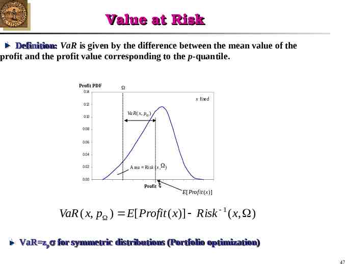
Value at Risk Definition: Definition: VaR is given by the difference between the mean value of the profit and the profit value corresponding to the p-quantile. Profit PDF 0.14 W x fixed 0.12 0.10 VaR ( x, p ) 0.08 0.06 0.04 0.02 Area Risk (x ,W ) 0.00 Profit x E[ Profit ( x )] VaR ( x, p ) E[ Profit ( x)] Risk 1 ( x, ) VaR zpp for for symmetric symmetric distributions (Portfolio optimization) 47
COMPUTATIONAL APPROACHES Sampling Average Approximation Method: Solve M times the problem using only N scenarios. If multiple solutions are obtained, use the first stage variables to solve the problem with a large number of scenarios N’ N to determine the optimum. Generalized Benders Decomposition Algorithm First Stage variables are complicating variables. This leaves a primal over second stage variables, which is decomposable. 48
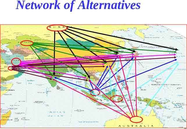
Example Generate a model to: Evaluate a large network of natural gas supplier-to-market transportation alternatives Identify the most profitable alternative(s) Manage financial risk 2005 2030 49
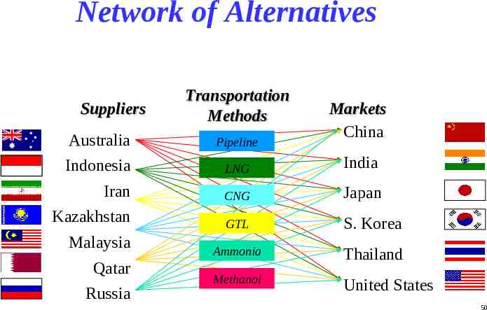
Network of Alternatives Suppliers Transportation Methods Markets China Australia Pipeline Indonesia LNG India Iran CNG Japan Kazakhstan GTL S. Korea Ammonia Thailand Methanol United States Malaysia Qatar Russia 50
Network of Alternatives 51
Results Risk Management (Downside Risk): 1.0 1.0 Malaysia GTL 1s 4.666 0.9 0.9 0.8 0.8 0.7 0.7 DR-200s 0.6 Mala-GTL 4.640 Ships: 4 & 2 ENPV:4.570 DR@ 4: 0.157 DR@ 3.5: 0.058 0.6 0.5 0.5 0.40.4 0.30.3 Indo-GTL 200s Ships: 5&3 4.678 ENPV:4.633 DR@ 4: 0.190 DR@ 3.5: 0.086 0.20.2 Thailand China 0.10.1 0.00.0 0 0 1 1 2 2 3 3 44 55 66 77 88 99 10 10 52
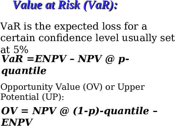
Value at Risk (VaR): VaR is the expected loss for a certain confidence level usually set at 5% VaR ENPV – NPV @ pquantile Opportunity Value (OV) or Upper Potential (UP): OV NPV @ (1-p)-quantile – ENPV 53
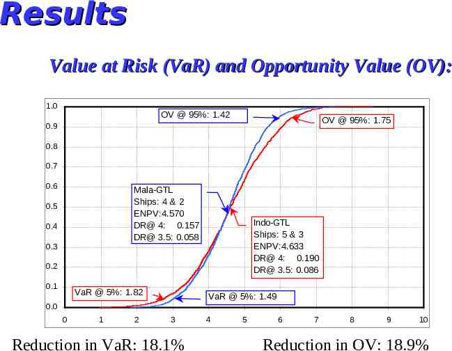
Results Value at Risk (VaR) and Opportunity Value (OV): 1.0 OV @ 95%: 1.42 OV @ 95%: 1.75 0.9 0.8 0.7 0.6 Mala-GTL Ships: 4 & 2 ENPV:4.570 DR@ 4: 0.157 DR@ 3.5: 0.058 0.5 0.4 0.3 Indo-GTL Ships: 5 & 3 ENPV:4.633 DR@ 4: 0.190 DR@ 3.5: 0.086 0.2 0.1 VaR @ 5%: 1.82 VaR @ 5%: 1.49 0.0 0 1 2 3 Reduction in VaR: 18.1% 4 5 6 7 8 9 10 Reduction in OV: 18.9% 54
Results Risk /Upside Potential Loss Ratio 1.0 OV @ 95%: 1.42 OV @ 95%: 1.75 0.9 0.8 0.7 O-Area: 0.116 0.6 Mala-GTL Ships: 4 & 2 ENPV:4.570 DR@ 4: 0.157 DR@ 3.5: 0.058 0.5 0.4 0.3 Indo-GTL Ships: 5 & 3 ENPV:4.633 DR@ 4: 0.190 DR@ 3.5: 0.086 R-Area: 0.053 0.2 0.1 VaR @ 5%: 1.82 VaR @ 5%: 1.49 0.0 0 1 2 3 4 5 6 Risk /Upside Potential Loss 7 8 9 10 55
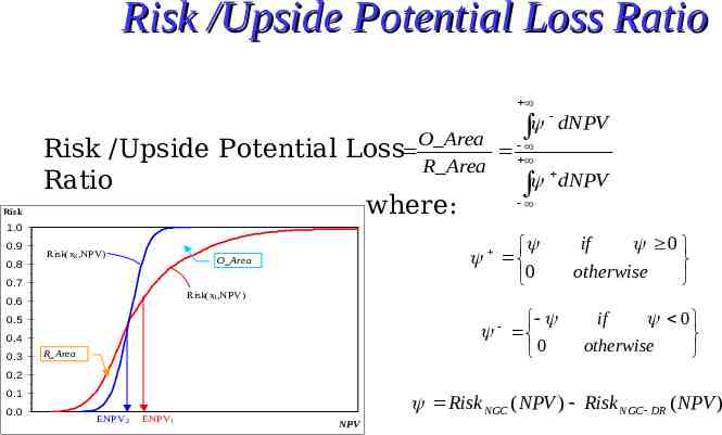
Risk /Upside Potential Loss Ratio dNPV Risk /Upside Potential Loss O Area R Area Ratio where: Risk dNPV 1.0 0.9 Risk(x2,NPV) 0.8 0 O Area 0.7 if 0 otherwise Risk(x1,NPV) 0.6 0 0.5 0.4 R Area 0.3 if 0 otherwise 0.2 0.1 0.0 0 1 ENPV2 2 3 ENPV1 4 Risk NGC ( NPV ) Risk NGC DR ( NPV ) 5 6 7 8 9 NPV 10 56
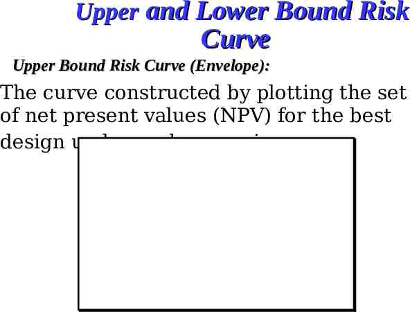
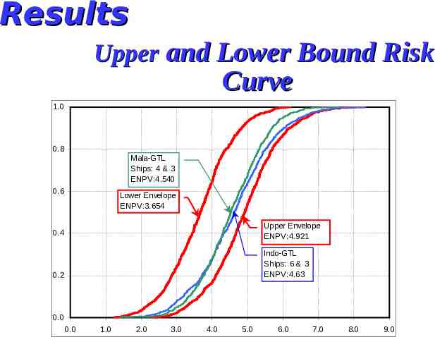
Upper and Lower Bound Risk Curve Upper Bound Risk Curve (Envelope): The curve constructed by plotting the set of net present values (NPV) for the best design under each scenario. Risk 1 a) Possible 0.8 b) Possible c) Impossible 0.6 E) Envelope 0.4 0.2 d) Impossible 0 0.00 0.0 2.00 2.0 4.00 4.0 6.00 6.0 8.00 8.0 10.00 10.0 57
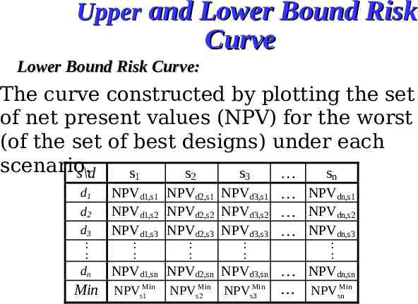
Upper and Lower Bound Risk Curve Lower Bound Risk Curve: The curve constructed by plotting the set of net present values (NPV) for the worst (of the set of best designs) under each scenario. s\d s1 s2 s3 sn d1 d2 d3 : : dn NPVd1,s1 NPVd2,s1 NPVd3,s1 NPVdn,s1 NPVd1,s2 NPVd2,s2 NPVd3,s2 NPVdn,s2 NPVd1,s3 NPVd2,s3 NPVd3,s3 NPVdn,s3 : : : : : : : : NPVd1,sn NPVd2,sn NPVd3,sn NPVdn,sn Min NPVs1Min NPVs2Min NPVs3Min NPVsnMin 58
Results Upper and Lower Bound Risk Curve 1.0 0.8 Mala-GTL Ships: 4 & 3 ENPV:4.540 0.6 Lower Envelope ENPV:3.654 0.4 Upper Envelope ENPV:4.921 0.2 Indo-GTL Ships: 6 & 3 ENPV:4.63 0.0 0.0 1.0 2.0 3.0 4.0 5.0 6.0 7.0 8.0 9.0 59
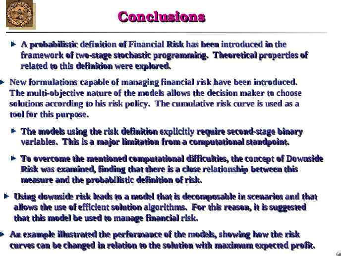
Conclusions A A probabilistic probabilistic definition of Financial Risk has been introduced in the framework framework of of two-stage two-stage stochastic stochastic programming. programming. Theoretical Theoretical properties properties of of related related to to this this definition definition were were explored. explored. New formulations capable of managing financial risk have been introduced. The multi-objective nature of the models allows the decision maker to choose solutions according to his risk policy. The cumulative risk curve is used as a tool for this purpose. The models using the the risk definition explicitly explicitly require require second-stage second-stage binary variables. This is a major limitation from a computational standpoint. To overcome the mentioned mentioned computational computational difficulties, difficulties, the the concept concept of of Downside Downside Risk was examined, finding that there is a close relationship between this measure and the probabilistic definition of risk. Using downside risk leads to a model that is decomposable in scenarios and that allows the use of efficient solution algorithms. For this reason, it is suggested suggested that this model be used used to to manage manage financial financial risk. risk. An An example example illustrated the performance of the models, showing how the risk curves curves can can be be changed changed in in relation relation to to the the solution solution with with maximum maximum expected expected profit. 60