Excel Lesson 6 Enhancing a Worksheet Microsoft Office

Excel Lesson 6 Enhancing a Worksheet Microsoft Office 2010 Introductory 1 Pasewark & Pasewark

Objectives Excel Lesson 6 Sort and filter data in a worksheet. Apply conditional formatting to highlight data. Hide worksheet columns and rows. Insert a shape, SmartArt graphic, picture, and screenshot in a worksheet. Use a template to create a new workbook. 2 Pasewark & Pasewark Microsoft Office 2010 Introductory

Objectives (continued) Excel Lesson 6 Insert a hyperlink in a worksheet. Save a workbook in a different file format. Insert, edit, and delete comments in a worksheet. Use the Research task pane. 3 Pasewark & Pasewark Microsoft Office 2010 Introductory

Sorting Data Excel Lesson 6 Sorting rearranges data in a more meaningful order. In an ascending sort, data with letters is arranged in alphabetical order (A to Z), numbers are arranged from smallest to largest. The reverse order occurs in a descending sort. 4 Pasewark & Pasewark Microsoft Office 2010 Introductory

Sorting Data Descending Excel Lesson 6 5 order sort arranges data with letters from Z to A, data with numbers from highest to lowest, and data with dates from oldest to newest. Pasewark & Pasewark Microsoft Office 2010 Introductory

Sorting Data When Excel Lesson 6 6 you sort data contained in columns of a worksheet, Excel does not include the column headings. To sort data, you first click a cell in the column by which you want to sort a range of data. Click the Data tab on the Ribbon. In the Sort and Filter group, click ascending or descending sort. Pasewark & Pasewark Microsoft Office 2010 Introductory

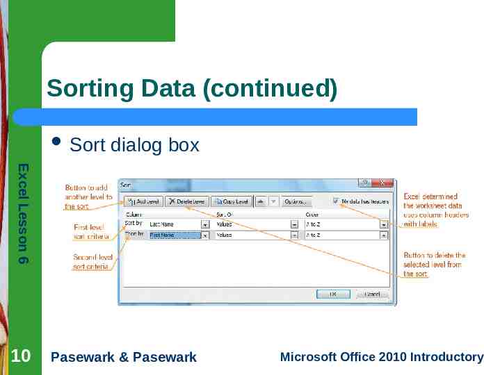
Sorting Data You Excel Lesson 6 7 can sort by more than one column of data. The columns will be sorted in order by the first-level sort criteria first, and then by the second-level sort criteria. Pasewark & Pasewark Microsoft Office 2010 Introductory

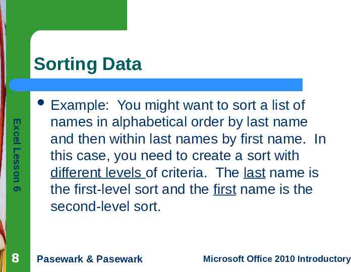
Sorting Data Example: Excel Lesson 6 8 You might want to sort a list of names in alphabetical order by last name and then within last names by first name. In this case, you need to create a sort with different levels of criteria. The last name is the first-level sort and the first name is the second-level sort. Pasewark & Pasewark Microsoft Office 2010 Introductory

Sorting Data If Excel Lesson 6 9 data is formatted with different font or fill colors, you can sort the data by color. Pasewark & Pasewark Microsoft Office 2010 Introductory

Sorting Data (continued) Sort dialog box Excel Lesson 6 10 Pasewark & Pasewark Microsoft Office 2010 Introductory

Filtering Data Filtering Excel Lesson 6 11 displays a subset of data that meets certain criteria and temporarily hides the rows that do not meet the specified criteria. You can filter by value, by criteria, or by color. Pasewark & Pasewark Microsoft Office 2010 Introductory

Filtering Data Filtering Excel Lesson 6 12 data will not remove errors. On the Data tab of the Ribbon, click the Filter button. Filter arrows appear in the lowerright corners of the cells with column headings. When you click a filter arrow, the AutoFilter menu for that column appears. Pasewark & Pasewark Microsoft Office 2010 Introductory

Filtering Data The Excel Lesson 6 13 AutoFilter menu displays a list of all the values that appear in that column along with additional criteria and color filtering options. When you want to see all the data in a worksheet again, you can restore all the rows by clearing the filter. Click the filter arrow and then click the Clear Filter From. Pasewark & Pasewark Microsoft Office 2010 Introductory

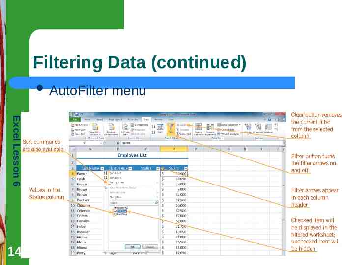
Filtering Data (continued) AutoFilter menu Excel Lesson 6 14 Pasewark & Pasewark Microsoft Office 2010 Introductory

Applying Conditional Formatting Conditional Excel Lesson 6 15 formatting changes the appearance of cells that meet a specified condition. To add conditional formatting, select the range you want to analyze. In the styles group on the Home tab, click the Conditional Formatting button. Pasewark & Pasewark Microsoft Office 2010 Introductory

Applying Conditional Formatting The Excel Lesson 6 16 Highlight Cells Rules format cells based on comparison operators such as greater than, less than, between, and equal to. – Highlights worksheet data by changing the look of cells that meet a specified condition. Pasewark & Pasewark Microsoft Office 2010 Introductory

Applying Conditional Formatting The Excel Lesson 6 17 Top/Bottom Rules format cells based on their rank, such as the top 10 items, above average or below average. Pasewark & Pasewark Microsoft Office 2010 Introductory

Hiding Columns and Rows Hiding Excel Lesson 6 18 a row or column temporarily removes it from view. Hiding rows and columns enables you to use the same worksheet to view different data. To hide data, select the rows or columns you want to hide, and then right-click the selection. On the shortcut menu that appears, click Hide. Pasewark & Pasewark Microsoft Office 2010 Introductory

Adding a Shape to a Worksheet Shapes, Excel Lesson 6 19 such as rectangles, circles, and arrows can help make a worksheet more informative. To open the Shapes gallery, click the Insert tab on the Ribbon, and then in the Illustrations group, click the Shapes button. Pasewark & Pasewark Microsoft Office 2010 Introductory

Adding a Shape to a Worksheet You Excel Lesson 6 20 can make a perfect square or circle by pressing and holding the shift key as you drag in the worksheet to draw the shape. When the shape is selected, the Drawing Tools appears on the Ribbon and contain the Format contextual tab. Pasewark & Pasewark Microsoft Office 2010 Introductory

Adding a Shape to a Worksheet Shapes Excel Lesson 6 21 are inserted in the worksheet as objects. An object is anything that appears on the screen that you can select and work with as a whole. When you no longer need a shape or any other object in a worksheet, you can delete it. First, click the object to select it, then press the Delete key. Pasewark & Pasewark Microsoft Office 2010 Introductory

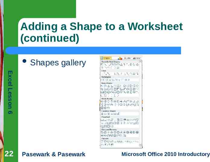
Adding a Shape to a Worksheet (continued) Shapes gallery Excel Lesson 6 22 Pasewark & Pasewark Microsoft Office 2010 Introductory

Adding a SmartArt Graphic to a Worksheet SmartArt Excel Lesson 6 23 graphics enhance worksheets by providing a visual representation of information and ideas. SmartArt graphics are often used for organizational charts, flowcharts, and decision trees. Pasewark & Pasewark Microsoft Office 2010 Introductory

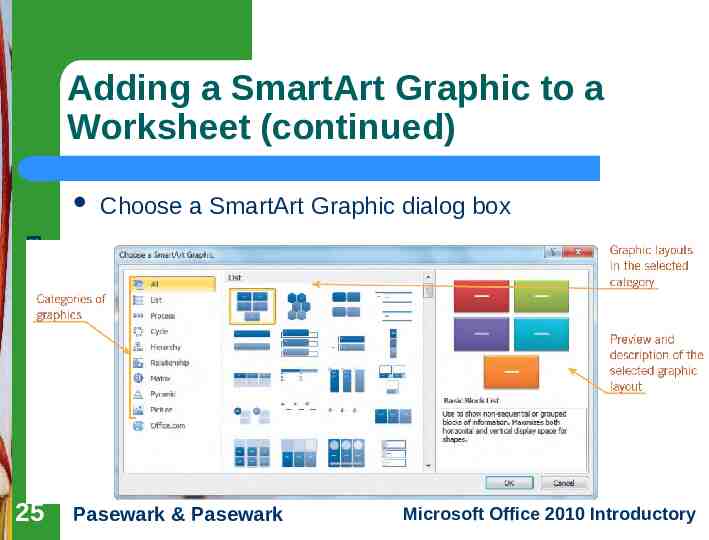
Adding a SmartArt Graphic to a Worksheet To Excel Lesson 6 24 insert a SmartArt graphic, click the SmartArt button in the Illustrations group on the Insert tab. The choose a SmartArt Graphic dialog box appears. When the SmartArt graphic is selected, SmartArt Tools appear on the Ribbon and contain the Design and Format contextual tabs. Pasewark & Pasewark Microsoft Office 2010 Introductory

Adding a SmartArt Graphic to a Worksheet (continued) Choose a SmartArt Graphic dialog box Excel Lesson 6 25 Pasewark & Pasewark Microsoft Office 2010 Introductory

Adding a Picture to a Worksheet A Excel Lesson 6 26 picture is a digital photograph or other image file. You can insert a picture in a worksheet by using a picture file, by using the Clip Art task pane, or from Office.com. Pasewark & Pasewark Microsoft Office 2010 Introductory

Adding a Picture to a Worksheet To Excel Lesson 6 27 insert a picture from a file, click the Picture button on the Illustrations group on the Insert tab of the Ribbon. A picture is inserted in the workbook as an object. As with shapes, you can move, resize, or format the picture to fit your needs. Pasewark & Pasewark Microsoft Office 2010 Introductory

Adding a Picture to a Worksheet The Excel Lesson 6 28 Format tab contains tools to edit and format the picture. If you want to adjust the brightness and contrast of a picture, you access the Format Contextual tab, and use the tools in the Adjust group to change the brightness and contrast. Pasewark & Pasewark Microsoft Office 2010 Introductory

Adding a Picture to a Worksheet If Excel Lesson 6 29 you want to change a picture’s shape and border, you access the Format Contextual tab and use the tools in the Picture Styles group to change the shape and color. Pasewark & Pasewark Microsoft Office 2010 Introductory

Adding a Picture to a Worksheet All Excel Lesson 6 30 images are protected by a copyright law. You cannot download and use a picture you find on a Website without permission. Some Web sites offer free images for noncommercial use. Others offer images you purchase for a fee. Pasewark & Pasewark Microsoft Office 2010 Introductory

Adding a Screenshot or Screen Clipping to a Worksheet A Excel Lesson 6 31 screenshot is a picture of all or part of something you see on your monitor. When you take a screenshot, you can include everything visible on your monitor or a screen clipping, which is the area you choose to include. Pasewark & Pasewark Microsoft Office 2010 Introductory

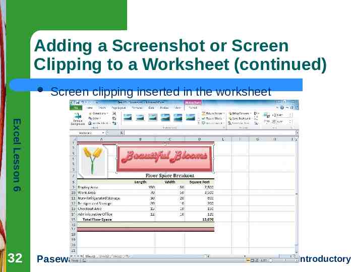
Adding a Screenshot or Screen Clipping to a Worksheet (continued) Screen clipping inserted in the worksheet Excel Lesson 6 32 Pasewark & Pasewark Microsoft Office 2010 Introductory

Using a Template Templates Excel Lesson 6 33 are predesigned workbook files that you can use as the basis or model for new workbooks. The template includes all the parts of a workbook that will not change, such as text labels, formulas, and formatting. Excel includes a variety of templates, which you access from the New tab in Backstage view. Pasewark & Pasewark Microsoft Office 2010 Introductory

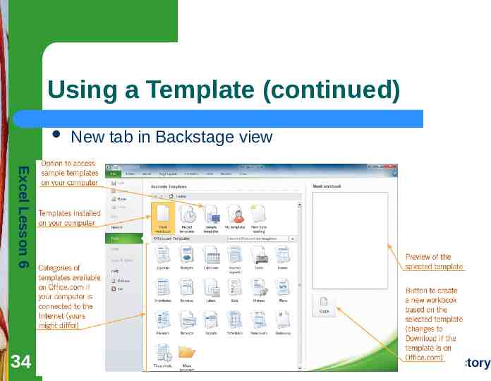
Using a Template (continued) New tab in Backstage view Excel Lesson 6 34 Pasewark & Pasewark Microsoft Office 2010 Introductory

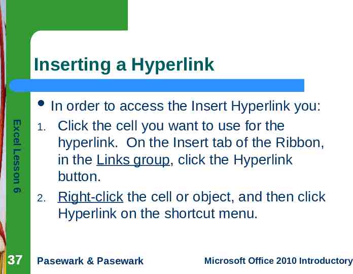
Inserting a Hyperlink A Excel Lesson 6 35 hyperlink is a reference in a workbook that opens another file or page when you click it. You can create hyperlinks that opens a Web page, a file, a specific location in the current workbook, a new document, or an e-mail address when you click it. Pasewark & Pasewark Microsoft Office 2010 Introductory

Inserting a Hyperlink The Excel Lesson 6 36 worksheet cell is the hyperlink, not the contents entered in that cell. To create or edit a hyperlink, you use the Hyperlink button on the Insert tab of the Ribbon. Pasewark & Pasewark Microsoft Office 2010 Introductory

Inserting a Hyperlink In Excel Lesson 6 37 1. 2. order to access the Insert Hyperlink you: Click the cell you want to use for the hyperlink. On the Insert tab of the Ribbon, in the Links group, click the Hyperlink button. Right-click the cell or object, and then click Hyperlink on the shortcut menu. Pasewark & Pasewark Microsoft Office 2010 Introductory

Inserting a Hyperlink Excel Lesson 6 38 3. In order to enter a ScreenTip to go with your Hyperlink, you would click Screen Tip in the dialog box. The Set Hyperlink Screen Tip Dialog Box will appear. Pasewark & Pasewark Microsoft Office 2010 Introductory

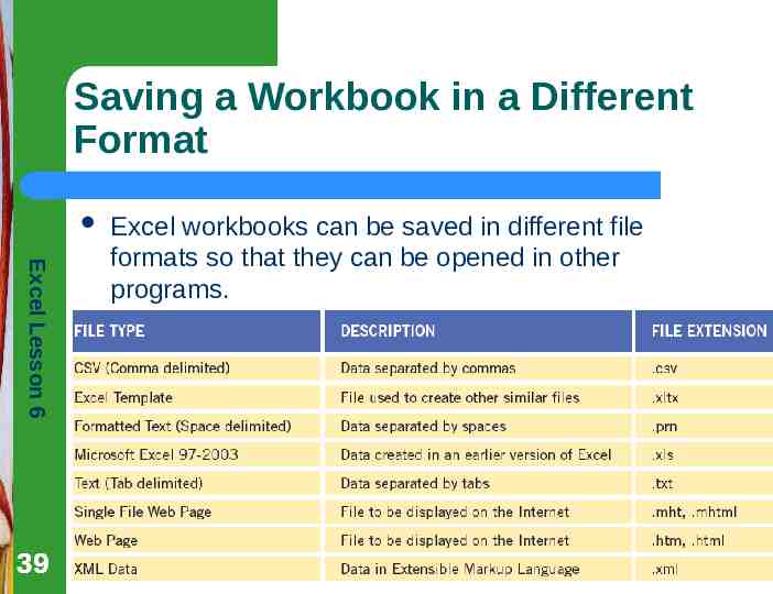
Saving a Workbook in a Different Format Excel Lesson 6 39 Excel workbooks can be saved in different file formats so that they can be opened in other programs. Pasewark & Pasewark Microsoft Office 2010 Introductory

Working with Comments A Excel Lesson 6 40 comment is a note attached to a cell that you can use to explain or identify information contained in the cell. All of the comments tools are located on the Review tab of the Ribbon. To edit a comment, click the cell that contains the comment. Then click the Edit Comment button on the Review tab. Pasewark & Pasewark Microsoft Office 2010 Introductory

Working with Comments Note: Excel Lesson 6 41 If you are working on another worksheet that belongs to someone else and you enter a comment, the username in the comment box will match the user name entered for that copy of Excel. If you want to change the username, click the File tab, and then click Options in the navigation bar. Pasewark & Pasewark Microsoft Office 2010 Introductory

Working with Comments You Excel Lesson 6 42 can show or hide all the comments in a worksheet by toggling the Show All comments button on the comments group. Pasewark & Pasewark Microsoft Office 2010 Introductory

Using the Research Task Pane The Research task pane provides access to information typically found in references such as dictionaries and encyclopedias. In Excel, the Research task pane also provides numerical data typically used in a worksheet, such as statistics or corporate financial data. To open the Research task pane, click the Review tab on the Ribbon, and then, in the Proofing group, click the Research button. Excel Lesson 6 43 Pasewark & Pasewark Microsoft Office 2010 Introductory

Using the Research Task Pane Excel Lesson 6 44 You can change which reference books and research sites are available from the Research task pane by clicking the Research options link at the bottom of the task pane. Pasewark & Pasewark Microsoft Office 2010 Introductory