EE 553 Introduction to Optimization J. McCalley 1


49 Slides1.56 MB
EE 553 Introduction to Optimization J. McCalley 1
Electricity markets and tools Day-ahead Real-time SCUC and SCED SCED BOTH LOOK LIKE THIS SCUC: x contains discrete & continuous variables. Minimize f(x) subject to h(x) c g(x) b SCED: x contains only continuous variables. 2
Optimization Terminology An optimization problem or a mathematical program or a mathematical programming problem. Minimize f(x) subject to h(x) c g(x) b f(x): Objective function x: Decision variables h(x) c: Equality constraint g(x) b: Inequality constraint x*: solution 3
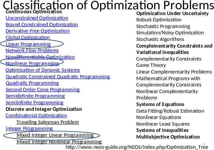
Classification of Optimization Problems Continuous Optimization Optimization Under Uncertainty Unconstrained Optimization Robust Optimization Bound Constrained Optimization Stochastic Programming Derivative-Free Optimization Simulation/Noisy Optimization Global Optimization Stochastic Algorithms Linear Programming Complementarity Constraints and Network Flow Problems Variational Inequalities Nondifferentiable Optimization Complementarity Constraints Nonlinear Programming Game Theory Optimization of Dynamic Systems Linear Complementarity Problems Quadratic Constrained Quadratic Programming Mathematical Programs with Quadratic Programming Complementarity Constraints Second Order Cone Programming Nonlinear Complementarity Semidefinite Programming Problems Semiinfinite Programming Systems of Equations Discrete and Integer Optimization Data Fitting/Robust Estimation Combinatorial Optimization Nonlinear Equations Traveling Salesman Problem Nonlinear Least Squares Integer Programming Systems of Inequalities Mixed Integer Linear Programming Multiobjective Optimization Mixed Integer Nonlinear Programming 4 http://www.neos-guide.org/NEOS/index.php/Optimization Tree
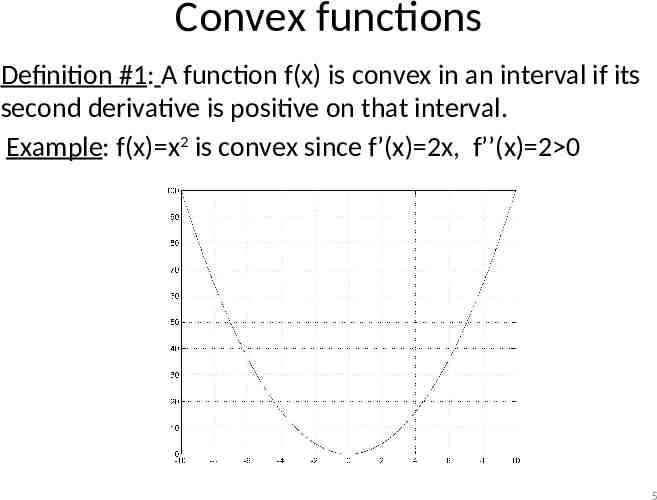
Convex functions Definition #1: A function f(x) is convex in an interval if its second derivative is positive on that interval. Example: f(x) x2 is convex since f’(x) 2x, f’’(x) 2 0 5
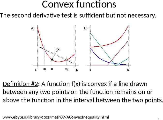
Convex functions The second derivative test is sufficient but not necessary. Definition #2: A function f(x) is convex if a line drawn between any two points on the function remains on or above the function in the interval between the two points. www.ebyte.it/library/docs/math09/AConvexInequality.html 6
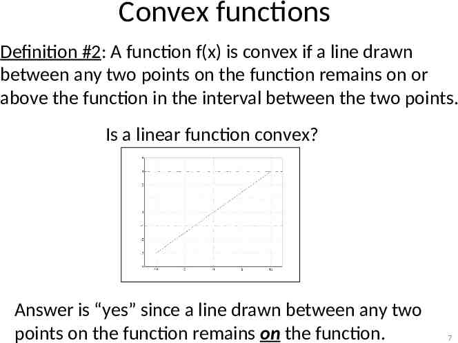
Convex functions Definition #2: A function f(x) is convex if a line drawn between any two points on the function remains on or above the function in the interval between the two points. Is a linear function convex? Answer is “yes” since a line drawn between any two points on the function remains on the function. 7
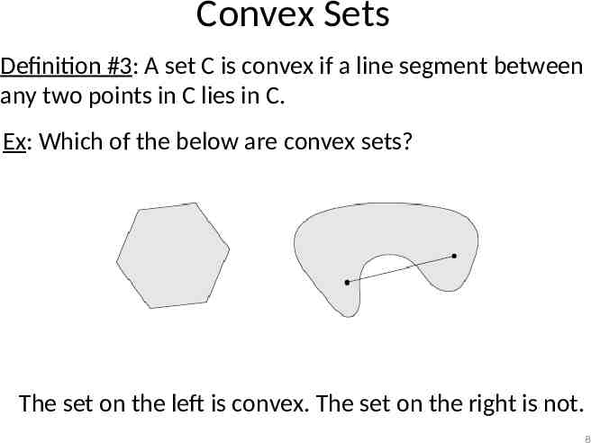
Convex Sets Definition #3: A set C is convex if a line segment between any two points in C lies in C. Ex: Which of the below are convex sets? The set on the left is convex. The set on the right is not. 8
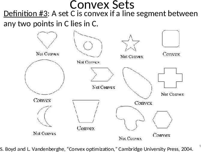
Convex Sets Definition #3: A set C is convex if a line segment between any two points in C lies in C. S. Boyd and L. Vandenberghe, “Convex optimization,” Cambridge University Press, 2004. 9
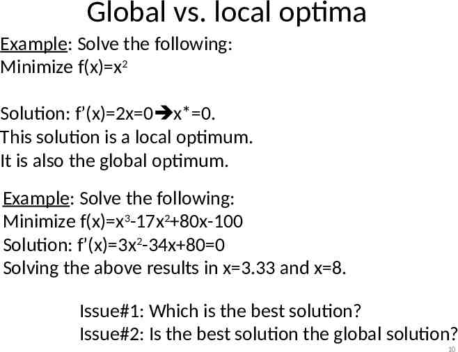
Global vs. local optima Example: Solve the following: Minimize f(x) x2 Solution: f’(x) 2x 0 x* 0. This solution is a local optimum. It is also the global optimum. Example: Solve the following: Minimize f(x) x3-17x2 80x-100 Solution: f’(x) 3x2-34x 80 0 Solving the above results in x 3.33 and x 8. Issue#1: Which is the best solution? Issue#2: Is the best solution the global solution? 10
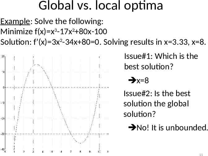
Global vs. local optima Example: Solve the following: Minimize f(x) x3-17x2 80x-100 Solution: f’(x) 3x2-34x 80 0. Solving results in x 3.33, x 8. Issue#1: Which is the best solution? x 8 Issue#2: Is the best solution the global solution? No! It is unbounded. 11
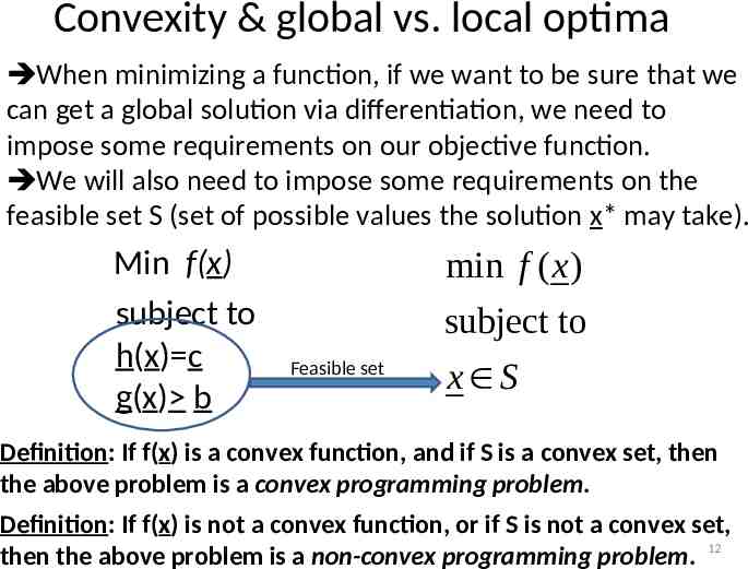
Convexity & global vs. local optima When minimizing a function, if we want to be sure that we can get a global solution via differentiation, we need to impose some requirements on our objective function. We will also need to impose some requirements on the feasible set S (set of possible values the solution x* may take). Min f(x) subject to h(x) c g(x) b min f ( x) subject to Feasible set x S Definition: If f(x) is a convex function, and if S is a convex set, then the above problem is a convex programming problem. Definition: If f(x) is not a convex function, or if S is not a convex set, then the above problem is a non-convex programming problem. 12
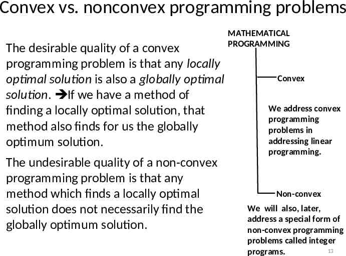
Convex vs. nonconvex programming problems The desirable quality of a convex programming problem is that any locally optimal solution is also a globally optimal solution. If we have a method of finding a locally optimal solution, that method also finds for us the globally optimum solution. The undesirable quality of a non-convex programming problem is that any method which finds a locally optimal solution does not necessarily find the globally optimum solution. MATHEMATICAL PROGRAMMING Convex We address convex programming problems in addressing linear programming. Non-convex We will also, later, address a special form of non-convex programming problems called integer 13 programs.
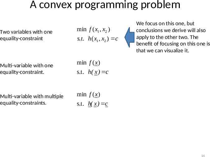
A convex programming problem Two variables with one equality-constraint Multi-variable with one equality-constraint. Multi-variable with multiple equality-constraints. min f ( x1 , x2 ) s.t. h( x1 , x2 ) c We focus on this one, but conclusions we derive will also apply to the other two. The benefit of focusing on this one is that we can visualize it. min f ( x) s.t. h( x ) c min f ( x) s.t. h( x ) c 14
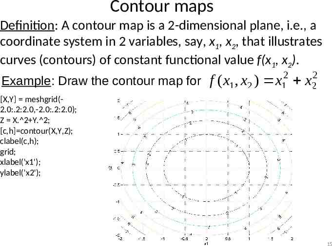
Contour maps Definition: A contour map is a. 2-dimensional plane, i.e., a coordinate system in 2 variables, say, x1, x2, that illustrates curves (contours) of constant functional value f(x1, x2). Example: Draw the contour map for f ( x1 , x2 ) 2 x1 2 x2 [X,Y] meshgrid(2.0:.2:2.0,-2.0:.2:2.0); Z X. 2 Y. 2; [c,h] contour(X,Y,Z); clabel(c,h); grid; xlabel('x1'); ylabel('x2'); 15
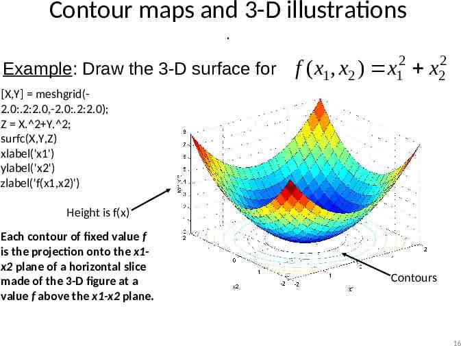
Contour maps and 3-D illustrations . Example: Draw the 3-D surface for f ( x1 , x2 ) 2 x1 2 x2 [X,Y] meshgrid(2.0:.2:2.0,-2.0:.2:2.0); Z X. 2 Y. 2; surfc(X,Y,Z) xlabel('x1') ylabel('x2') zlabel('f(x1,x2)') Height is f(x) Each contour of fixed value f is the projection onto the x1x2 plane of a horizontal slice made of the 3-D figure at a value f above the x1-x2 plane. Contours 16
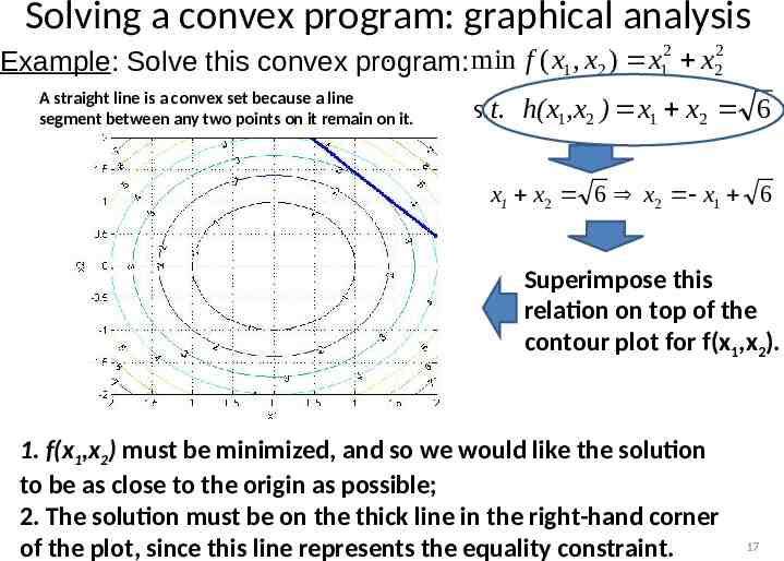
Solving a convex program: graphical analysis Example: Solve this convex . min program: A straight line is a convex set because a line segment between any two points on it remain on it. f ( x1 , x2 ) x12 x22 s.t. h(x1,x2 ) x1 x2 6 x1 x2 6 x2 x1 6 Superimpose this relation on top of the contour plot for f(x1,x2). 1. f(x1,x2) must be minimized, and so we would like the solution to be as close to the origin as possible; 2. The solution must be on the thick line in the right-hand corner of the plot, since this line represents the equality constraint. 17
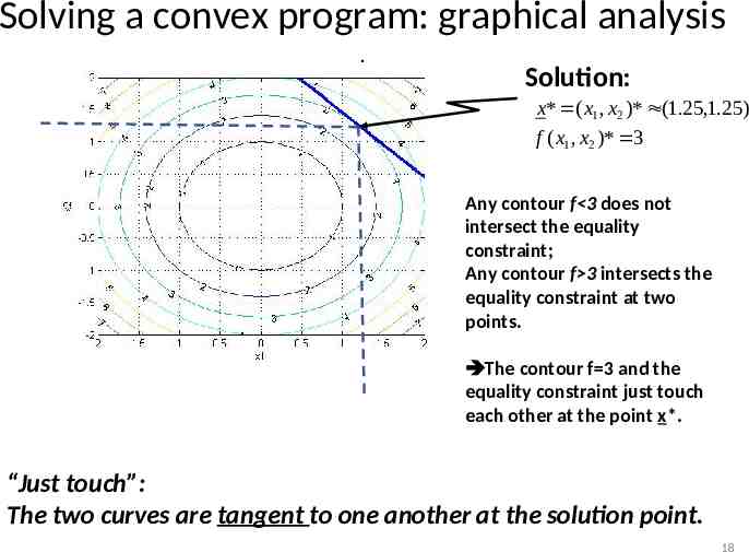
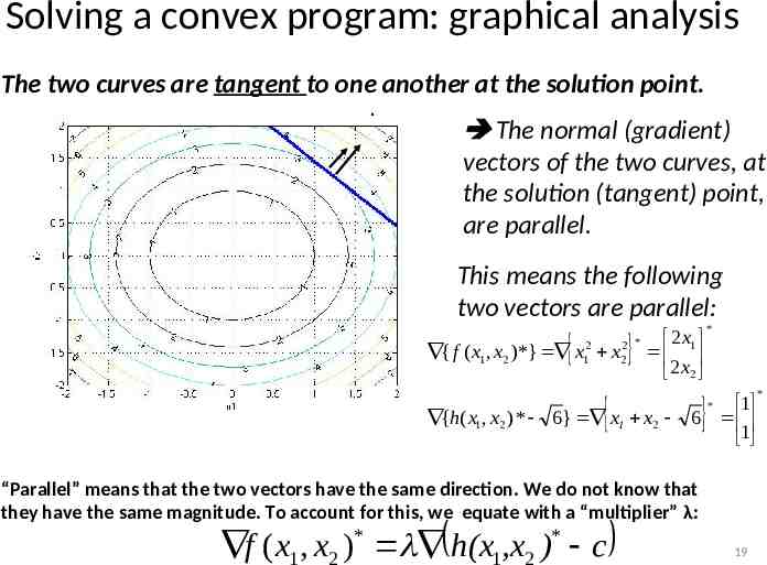
Solving a convex program: graphical analysis . Solution: x* ( x1 , x2 )* (1.25,1.25) f ( x1 , x2 )* 3 Any contour f 3 does not intersect the equality constraint; Any contour f 3 intersects the equality constraint at two points. The contour f 3 and the equality constraint just touch each other at the point x*. “Just touch”: The two curves are tangent to one another at the solution point. 18
Solving a convex program: graphical analysis The two curves are tangent to one another at the solution point. . The normal (gradient) vectors of the two curves, at the solution (tangent) point, are parallel. This means the following two vectors are parallel: { f ( x1 , x2 )*} x12 x 2 * 2 2x 1 2 x2 {h( x1 , x2 ) * 6} x1 x2 1 6 1 “Parallel” means that the two vectors have the same direction. We do not know that they have the same magnitude. To account for this, we equate with a “multiplier” λ: * * 1 2 1 2 f ( x , x ) h(x ,x ) c * * 19 *
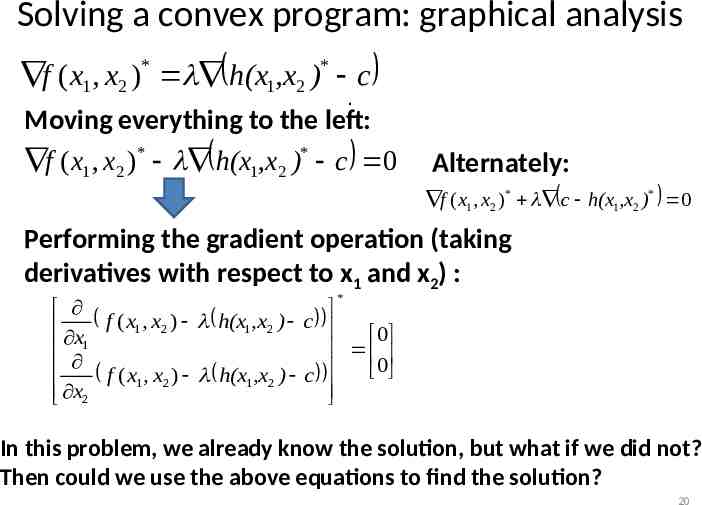
Solving a convex program: graphical analysis * * f ( x1 , x2 ) h(x1,x2 ) c . Moving everything to the left: f ( x1 , x2 )* h(x1,x2 )* c 0 Alternately: f ( x1 , x2 )* c h(x1,x2 )* 0 Performing the gradient operation (taking derivatives with respect to x1 and x2) : * f ( x , x ) h(x ,x ) c 1 2 1 2 x 0 1 f ( x , x ) h(x ,x ) c 0 1 2 1 2 x2 In this problem, we already know the solution, but what if we did not? Then could we use the above equations to find the solution? 20
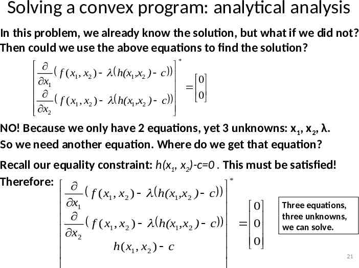
Solving a convex program: analytical analysis In this problem, we already know the solution, but what if we did not? Then could we use the above equations to find the solution? * f ( x , x ) h(x ,x ) c 1 2 1 2 x 0 1 f ( x1 , x2 ) h(x1,x2 ) c 0 x2 NO! Because we only have 2 equations, yet 3 unknowns: x1, x2, λ. So we need another equation. Where do we get that equation? Recall our equality constraint: h(x1, x2)-c 0 . This must be satisfied! * Therefore: f ( x , x ) h(x ,x ) c 1 2 1 2 x Three equations, 0 1 three unknowns, f ( x , x ) h(x ,x ) c 0 1 2 1 2 we can solve. x2 0 h( x1 , x2 ) c 21
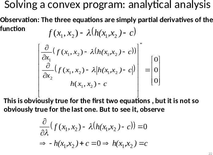
Solving a convex program: analytical analysis Observation: The three equations are simply partial derivatives of the function f ( x1 , x2 ) h(x1 ,x2 ) c * x f ( x1 , x2 ) h(x1,x2 ) c 0 1 f ( x , x ) h(x ,x ) c 0 1 2 1 2 x2 0 h( x1 , x2 ) c This is obviously true for the first two equations , but it is not so obviously true for the last one. But to see it, observe f ( x1 , x2 ) h(x1,x2 ) c 0 h(x1,x2 ) c 0 h(x1,x2 ) c 22
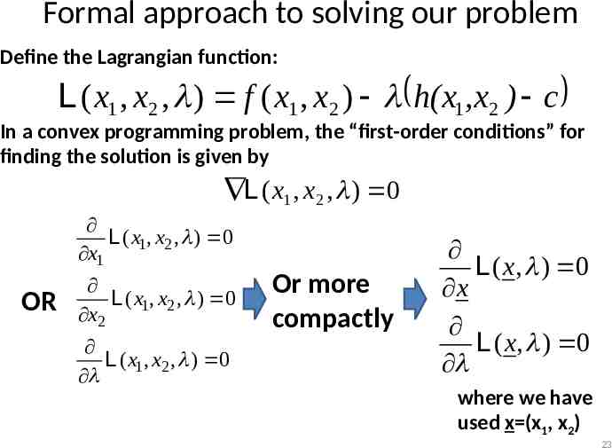
Formal approach to solving our problem Define the Lagrangian function: L ( x1 , x2 , ) f ( x1 , x2 ) h(x1 ,x2 ) c In a convex programming problem, the “first-order conditions” for finding the solution is given by L ( x1 , x2 , ) 0 L ( x1, x2 , ) 0 x1 OR L ( x1, x2 , ) 0 x2 L ( x1, x2 , ) 0 Or more compactly L ( x, ) 0 x L ( x, ) 0 where we have used x (x1, x2) 23
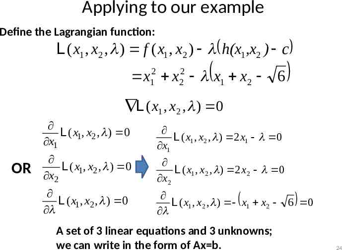
Applying to our example Define the Lagrangian function: L ( x1 , x2 , ) f ( x1 , x2 ) h(x1,x2 ) c 2 1 2 2 x x x1 x2 6 L ( x1 , x2 , ) 0 OR L ( x1, x2 , ) 0 x1 L ( x1 , x2 , ) 2 x1 0 x1 L ( x1, x2 , ) 0 x2 L ( x1 , x2 , ) 2 x2 0 x2 L ( x1, x2 , ) 0 L ( x1 , x 2 , ) x1 x2 A set of 3 linear equations and 3 unknowns; we can write in the form of Ax b. 6 0 24
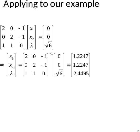
Applying to our example 2 0 1 x1 0 0 2 1 x 0 2 1 1 0 6 1 x1 2 0 1 0 1.2247 x2 0 2 1 0 1.2247 1 1 0 6 2.4495 25
Now, let’s go back to our example with a nonlinear equality constraint.
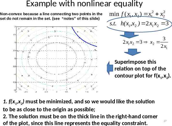
Example with nonlinear equality . in the Non-convex because a line connecting two points set do not remain in the set. (see “notes” of this slide) min f ( x1 , x2 ) x12 x22 s.t. h(x1,x2 ) 2 x1 x2 3 3 2 x1x2 3 x2 2 x1 Superimpose this relation on top of the contour plot for f(x1,x2). 1. f(x1,x2) must be minimized, and so we would like the solution to be as close to the origin as possible; 2. The solution must be on the thick line in the right-hand corner of the plot, since this line represents the equality constraint. 27
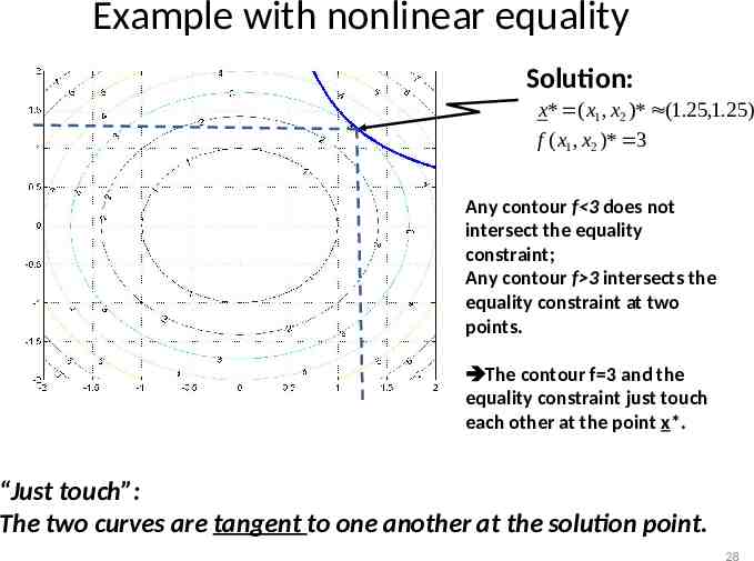
Example with nonlinear equality . Solution: x* ( x1 , x2 )* (1.25,1.25) f ( x1 , x2 )* 3 Any contour f 3 does not intersect the equality constraint; Any contour f 3 intersects the equality constraint at two points. The contour f 3 and the equality constraint just touch each other at the point x*. “Just touch”: The two curves are tangent to one another at the solution point. 28
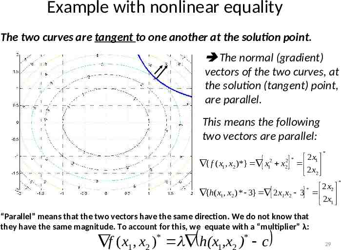
Example with nonlinear equality The two curves are tangent to one another at the solution point. . The normal (gradient) vectors of the two curves, at the solution (tangent) point, are parallel. This means the following two vectors are parallel: { f ( x1 , x2 )*} x12 x 2 * 2 2x 1 2 x2 * 2 x2 {h( x1 , x2 ) * 3} 2 x1 x2 3 2 x1 * “Parallel” means that the two vectors have the same direction. We do not know that they have the same magnitude. To account for this, we equate with a “multiplier” λ: * * 1 2 1 2 f ( x , x ) h(x ,x ) c 29 *
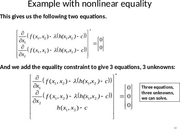
Example with nonlinear equality This gives us the following two equations. * f ( x , x ) h(x ,x ) c 1 2 1 2 x 0 1 f ( x1 , x2 ) h(x1,x2 ) c 0 x2 And we add the equality constraint to give 3 equations, 3 unknowns: * f ( x , x ) h(x ,x ) c 1 2 1 2 x 0 1 f ( x , x ) h(x ,x ) c 0 1 2 1 2 x2 0 h( x1 , x2 ) c Three equations, three unknowns, we can solve. 30
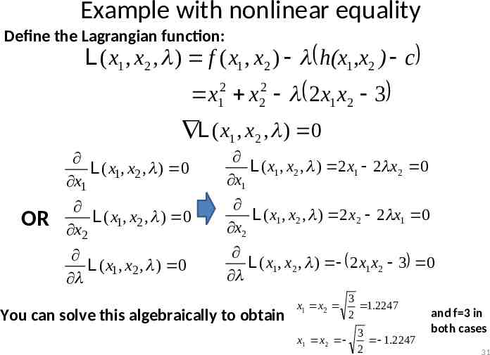
Example with nonlinear equality Define the Lagrangian function: L ( x1 , x2 , ) f ( x1 , x2 ) h(x1,x2 ) c 2 1 2 2 x x 2 x1 x2 3 L ( x1 , x2 , ) 0 OR L ( x1, x2 , ) 0 x1 L ( x1 , x2 , ) 2 x1 2 x2 0 x1 L ( x1, x2 , ) 0 x2 L ( x1 , x2 , ) 2 x2 2 x1 0 x2 L ( x1, x2 , ) 0 L ( x1 , x2 , ) 2 x1 x2 3 0 You can solve this algebraically to obtain x1 x2 x1 x 2 3 1.2247 2 3 1.2247 2 and f 3 in both cases 31
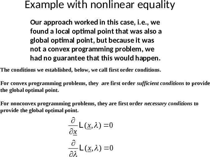
Example with nonlinear equality Our approach worked in this case, i.e., we found a local optimal point that was also a global optimal point, but because it was not a convex programming problem, we had no guarantee that this would happen. The conditions we established, below, we call first order conditions. For convex programming problems, they are first order sufficient conditions to provide the global optimal point. For nonconvex programming problems, they are first order necessary conditions to provide the global optimal point. L ( x, ) 0 x L ( x, ) 0
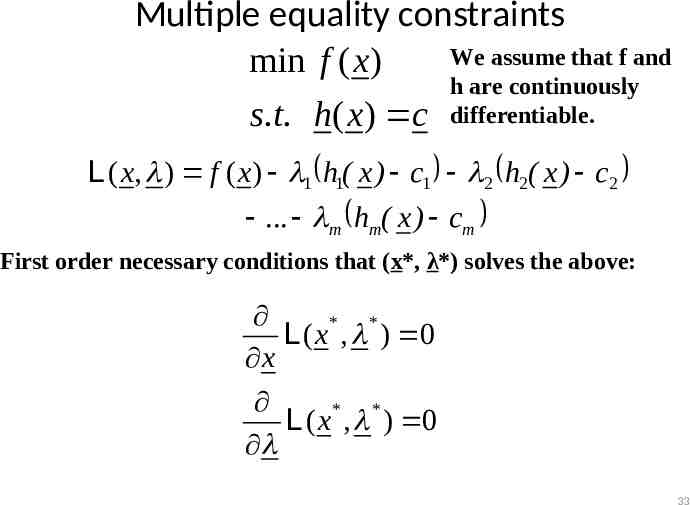
Multiple equality constraints We assume that f and min f ( x) h are continuously s.t. h( x) c differentiable. L ( x, ) f ( x) 1 h1( x ) c1 2 h2( x ) c2 . m hm( x ) cm First order necessary conditions that (x*, λ*) solves the above: * * L ( x , ) 0 x * * L ( x , ) 0 33
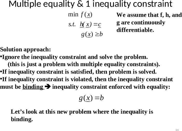
Multiple equality & 1 inequality constraint min f ( x) s.t. h( x ) c g ( x) b We assume that f, h, and g are continuously differentiable. Solution approach: Ignore the inequality constraint and solve the problem. (this is just a problem with multiple equality constraints). If inequality constraint is satisfied, then problem is solved. If inequality constraint is violated, then the inequality constraint must be binding inequality constraint enforced with equality: g ( x) b Let’s look at this new problem where the inequality is binding. 34
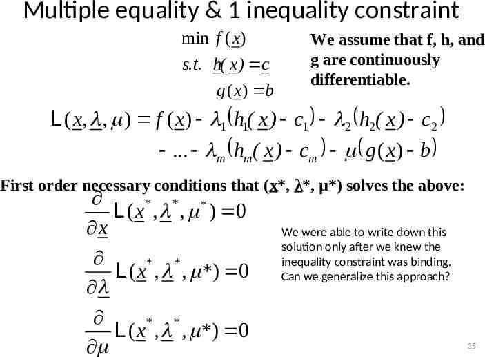
Multiple equality & 1 inequality constraint min f ( x) s.t. h( x ) c g ( x) b We assume that f, h, and g are continuously differentiable. L ( x, , ) f ( x) 1 h1( x ) c1 2 h2( x ) c2 . m hm( x ) cm g ( x) b First order necessary conditions that (x*, λ*, μ*) solves the above: * * L ( x , , * ) 0 x * * L ( x , , *) 0 * * L ( x , , *) 0 We were able to write down this solution only after we knew the inequality constraint was binding. Can we generalize this approach? 35
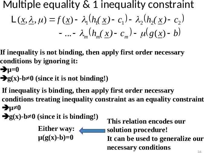
Multiple equality & 1 inequality constraint L ( x, , ) f ( x) 1 h1( x ) c1 2 h2( x ) c2 . m hm( x ) cm g ( x) b If inequality is not binding, then apply first order necessary conditions by ignoring it: μ 0 g(x)-b 0 (since it is not binding!) If inequality is binding, then apply first order necessary conditions treating inequality constraint as an equality constraint μ 0 g(x)-b 0 (since it is binding!) This relation encodes our Either way: solution procedure! μ(g(x)-b) 0 It can be used to generalize our necessary conditions 36
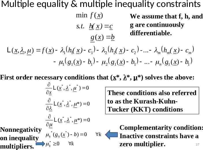
Multiple equality & multiple inequality constraints min f ( x) s.t. h( x ) c g ( x) b We assume that f, h, and g are continuously differentiable. L ( x, , ) f ( x) 1 h1( x ) c1 2 h2( x ) c2 - . m hm( x ) cm 1 g1 ( x) b1 2 g1 ( x) b1 . n g1 ( x) b1 First order necessary conditions that (x*, λ*, μ*) solves the above: * * * L ( x , , ) 0 x * * L ( x , , *) 0 * * L ( x , , *) 0 Nonnegativity * * k ( g k ( x ) b) 0 on inequality k* 0 k multipliers. These conditions also referred to as the Kurash-KuhnTucker (KKT) conditions k Complementarity condition: Inactive constraints have a 37 zero multiplier.
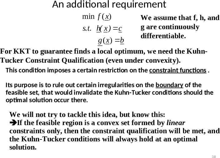
An additional requirement min f ( x) s.t. h( x ) c g ( x) b We assume that f, h, and g are continuously differentiable. For KKT to guarantee finds a local optimum, we need the KuhnTucker Constraint Qualification (even under convexity). This condition imposes a certain restriction on the constraint functions . Its purpose is to rule out certain irregularities on the boundary of the feasible set, that would invalidate the Kuhn-Tucker conditions should the optimal solution occur there. We will not try to tackle this idea, but know this: If the feasible region is a convex set formed by linear constraints only, then the constraint qualification will be met, and the Kuhn-Tucker conditions will always hold at an optimal solution. 38
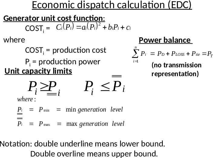
Economic dispatch calculation (EDC) Generator unit cost function: 2 C i P i a i P i biPi ci COSTi where Power balance n COSTi production cost Pi PD PLOSS Ptie PT i 1 Pi production power (no transmission Unit capacity limits representation) Pi P i Pi P i where : Pi P min min generation level Pi P max max generation level Notation: double underline means lower bound. Double overline means upper bound.
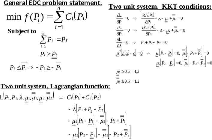
General EDC problem statement. Two unit system, KKT conditions: n min f ( Pi ) Ci Pi Subject to i 1 L C1 P1 0 1 1 0 P1 P1 L C 2 P 2 0 2 2 0 P 2 P 2 L 0 P1 P 2 PT 0 Pi Pi h x c 0 i 1 n P i PT k 0, k 1,2 Two unit system, Lagrangian function: 2 P 2 P 2 0, 2 P 2 P 2 0 Pi Pi Pi Pi L P1, P 2, , 1, 1, 2, 2 1 P1 P1 0, 1 P1 P1 0 k 0, k 1,2 C1 P1 C 2 P 2 P1 P2 PT 1 P1 P1 1 P1 P1 2 P2 P2 2 P2 P2
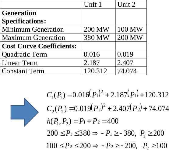
Generation Specifications: Minimum Generation Maximum Generation Cost Curve Coefficients: Quadratic Term Linear Term Constant Term Unit 1 Unit 2 200 MW 380 MW 100 MW 200 MW 0.016 2.187 120.312 0.019 2.407 74.074 2 C1 ( P1 ) 0.016 P1 2.187 P1 120.312 2 C2 ( P2 ) 0.019 P 2 2.407 P 2 74.074 h( P1 , P2 ) P1 P 2 400 200 P1 380 P1 380, P1 200 100 P 2 200 P 2 200, P2 100
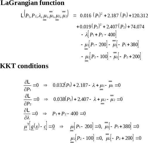
LaGrangian function L P1, P 2, , 1, 1, 2, 2 2 0.016 P1 2.187 P1 120.312 2 0.019 P 2 2.407 P 2 74.074 P1 P 2 400 1 P1 200 1 P1 380 2 P 2 100 2 P 2 200 KKT conditions L 0 0.032 P1 2.187 1 1 0 P1 L 0 0.038 P 2 2.407 2 2 0 P 2 L 0 P1 P 2 400 0 g x c 0 1 P1 200 0, 1 P1 380 0 2 P 2 100 0, 2 P 2 200 0
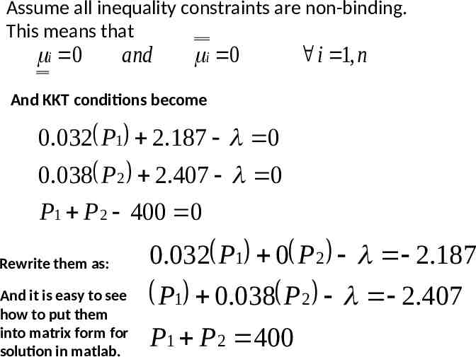
Assume all inequality constraints are non-binding. This means that i 0 and i 0 i 1, n And KKT conditions become 0.032 P1 2.187 0 0.038 P 2 2.407 0 P1 P 2 400 0 Rewrite them as: And it is easy to see how to put them into matrix form for solution in matlab. 0.032 P1 0 P 2 2.187 P1 0.038 P 2 2.407 P1 P 2 400
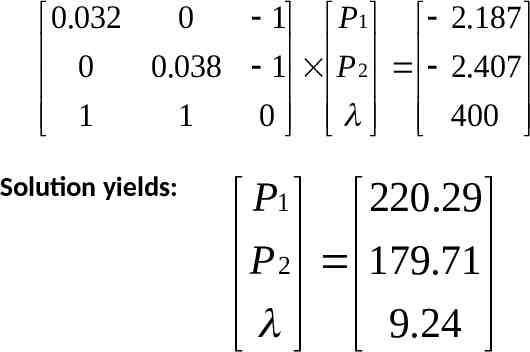
0 1 P1 2.187 0.032 0 0.038 1 P 2 2.407 1 1 0 400 Solution yields: P1 220.29 P 2 179.71 9.24
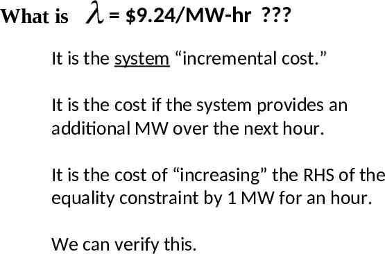
What is 9.24/MW-hr ? It is the system “incremental cost.” It is the cost if the system provides an additional MW over the next hour. It is the cost of “increasing” the RHS of the equality constraint by 1 MW for an hour. We can verify this.
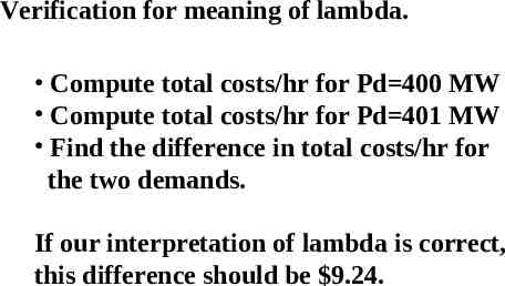
Verification for meaning of lambda. Compute total costs/hr for Pd 400 MW Compute total costs/hr for Pd 401 MW Find the difference in total costs/hr for the two demands. If our interpretation of lambda is correct, this difference should be 9.24.
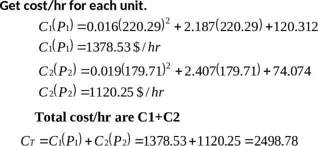
Get cost/hr for each unit. 2 C1 P1 0.016 220.29 2.187 220.29 120.312 C1 P1 1378.53 / hr 2 C 2 P 2 0.019 179.71 2.407 179.71 74.074 C 2 P 2 1120.25 / hr Total cost/hr are C1 C2 CT C1 P1 C 2 P 2 1378.53 1120.25 2498.78
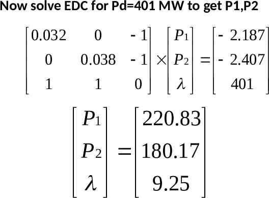
Now solve EDC for Pd 401 MW to get P1,P2 0 1 P1 2.187 0.032 0 0.038 1 P 2 2.407 1 1 0 401 P1 220.83 P 2 180.17 9.25
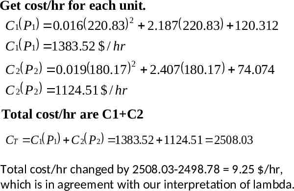
Get cost/hr for each unit. 2 C1 P1 0.016 220.83 2.187 220.83 120.312 C1 P1 1383.52 / hr 2 C 2 P 2 0.019 180.17 2.407 180.17 74.074 C 2 P 2 1124.51 / hr Total cost/hr are C1 C2 CT C1 P1 C 2 P 2 1383.52 1124.51 2508.03 Total cost/hr changed by 2508.03-2498.78 9.25 /hr, which is in agreement with our interpretation of lambda.