Doing data analysis with the multilevel model for change ALDA, Chapter
28 Slides1.95 MB
Doing data analysis with the multilevel model for change ALDA, Chapter Four “We are restless because of incessant change, but we would be frightened if change were stopped” Lyman Bryson Judith D. Singer & John B. Willett Harvard Graduate School of Education
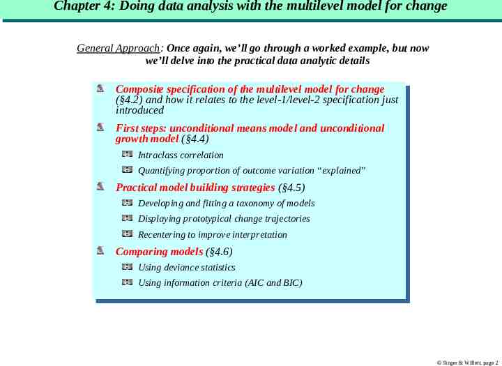
Chapter Chapter 4: 4: Doing Doing data data analysis analysis with with the the multilevel multilevel model model for for change change General Approach: Once again, we’ll go through a worked example, but now we’ll delve into the practical data analytic details Composite Compositespecification specificationofofthe themultilevel multilevelmodel modelfor forchange change (§4.2) and how it relates to the level-1/level-2 specification (§4.2) and how it relates to the level-1/level-2 specificationjust just introduced introduced First Firststeps: steps:unconditional unconditionalmeans meansmodel modeland andunconditional unconditional growth model (§4.4) growth model (§4.4) Intraclass Intraclasscorrelation correlation Quantifying Quantifyingproportion proportionofofoutcome outcomevariation variation“explained” “explained” Practical Practicalmodel modelbuilding buildingstrategies strategies(§4.5) (§4.5) Developing Developingand andfitting fittingaataxonomy taxonomyofofmodels models Displaying Displayingprototypical prototypicalchange changetrajectories trajectories Recentering Recenteringtotoimprove improveinterpretation interpretation Comparing Comparingmodels models(§4.6) (§4.6) Using Usingdeviance deviancestatistics statistics Using Usinginformation informationcriteria criteria(AIC (AICand andBIC) BIC) Singer & Willett, page 2
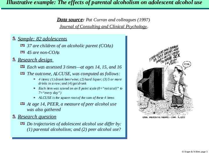
Illustrative Illustrative example: example: The The effects effects of of parental parental alcoholism alcoholism on on adolescent adolescent alcohol alcohol use use Data source: Pat Curran and colleagues (1997) Journal of Consulting and Clinical Psychology. Sample: Sample:82 82adolescents adolescents 37 37are arechildren childrenofofan analcoholic alcoholicparent parent(COAs) (COAs) 45 45are arenon-COAs non-COAs Research Researchdesign design Each Eachwas wasassessed assessed33times—at times—atages ages14, 14,15, 15,and and16 16 The Theoutcome, outcome,ALCUSE, ALCUSE,was wascomputed computedas asfollows: follows: 44items: items:(1) (1)drank drankbeer/wine; beer/wine;(2) (2)hard hardliquor; liquor;(3) (3)55orormore more drinks in a row; and (4) got drunk drinks in a row; and (4) got drunk Each item was scored on an 8 point scale (0 “not at all” to Each item was scored on an 8 point scale (0 “not at all” to 7 “every day”) 7 “every day”) ALCUSE is the square root of the sum of these 4 items ALCUSE is the square root of the sum of these 4 items At Atage age14, 14,PEER, PEER,aameasure measureofofpeer peeralcohol alcoholuse use was also gathered was also gathered Research Researchquestion question Do Dotrajectories trajectoriesofofadolescent adolescentalcohol alcoholuse usediffer differby: by: (1) (1)parental parentalalcoholism; alcoholism;and and(2) (2)peer peeralcohol alcoholuse? use? Singer & Willett, page 3
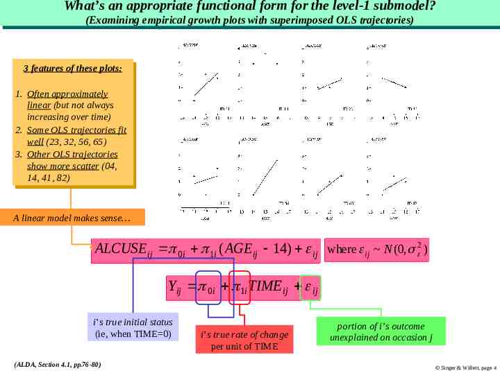
What’s What’s an an appropriate appropriate functional functional form form for for the the level-1 level-1 submodel? submodel? (Examining (Examiningempirical empiricalgrowth growthplots plotswith withsuperimposed superimposedOLS OLStrajectories) trajectories) 33features featuresof ofthese theseplots: plots: 1.1. Often Oftenapproximately approximately linear (but linear (butnot notalways always increasing over increasing overtime) time) 2.2. Some SomeOLS OLStrajectories trajectoriesfit fit well (23, 32, 56, 65) well (23, 32, 56, 65) 3.3. Other OtherOLS OLStrajectories trajectories show more scatter show more scatter(04, (04, 14, 41, 82) 14, 41, 82) A linear model makes sense ALCUSE ij 0i 1i ( AGE ij 14) ij where ij N (0, 2 ) Yij 0i 1i TIMEij ij i’s true initial status (ie, when TIME 0) (ALDA, Section 4.1, pp.76-80) i’s true rate of change per unit of TIME portion of i’s outcome unexplained on occasion j Singer & Willett, page 4
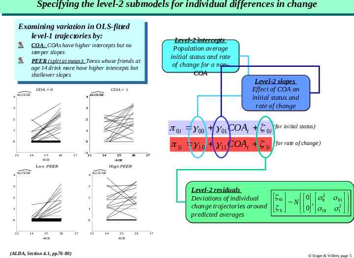
Specifying Specifying the the level-2 level-2 submodels submodels for for individual individual differences differences in in change change Examining Examiningvariation variationininOLS-fitted OLS-fitted level-1 level-1trajectories trajectoriesby: by: Level-2 intercepts Population average initial status and rate of change for a nonCOA COA: COAs have higher intercepts but no COA: COAs have higher intercepts but no steeper slopes steeper slopes PEER PEER(split (splitatatmean): mean):Teens Teenswhose whosefriends friendsatat age age1414drink drinkmore morehave havehigher higherintercepts interceptsbut but shallower slopes shallower slopes COA 1 COA 0 4 ALCUSE 4 3 3 2 2 1 1 0 0 -1 13 14 15 AGE 16 17 ALCUSE 0i 00 01COAi 0i (for initial status) 1i 10 11COAi 1i -1 13 14 Low PEER 4 4 3 3 2 2 1 1 0 0 14 15 AGE 15 AGE 16 (for rate of change) 17 High PEER ALCUSE -1 13 Level-2 slopes Effect of COA on initial status and rate of change 16 (ALDA, Section 4.1, pp.76-80) 17 ALCUSE -1 13 Level-2 residuals Deviations of individual change trajectories around predicted averages 14 15 AGE 16 0 022 01 00ii 0 01 N 0 , 22 11ii 10 1 10 1 17 Singer & Willett, page 5
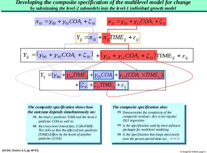
Developing Developing the the composite composite specification specification of of the the multilevel multilevel model model for for change change by bysubstituting substitutingthe thelevel-2 level-2submodels submodelsinto intothe thelevel-1 level-1individual individualgrowth growthmodel model 0i 00 01COAi 0i 1i 10 11COAi 1i Yij 0i 1i TIME ij ij Yij 00 01COAi 0i 10 11COAi 1i TIME ij ij Yij [ 00 10TIME ij 01COAi 11 (COAi TIME ij )] [ 0i 1i TIME ij ij ] The Thecomposite compositespecification specificationshows showshow how the outcome depends simultaneously the outcome depends simultaneouslyon: on: the thelevel-1 level-1predictor predictorTIME TIMEand andthe thelevel-2 level-2 predictor COA as well as predictor COA as well as the cross-level interaction, COA TIME. the cross-level interaction, COA TIME. This tells us that the effect of one predictor This tells us that the effect of one predictor (TIME) differs by the levels of another (TIME) differs by the levels of another predictor (COA) predictor (COA) (ALDA, Section 4.2, pp. 80-83) The Thecomposite compositespecification specificationalso: also: Demonstrates the complexity of the Demonstrates the complexity of the composite residual—this is not regular composite residual—this is not regular OLS regression OLS regression Is the specification used by most software Is the specification used by most software packages for multilevel modeling packages for multilevel modeling IsIsthe thespecification specificationthat thatmaps mapsmost mosteasily easily onto ontothe theperson-period person-perioddata dataset set Singer & Willett, page 6
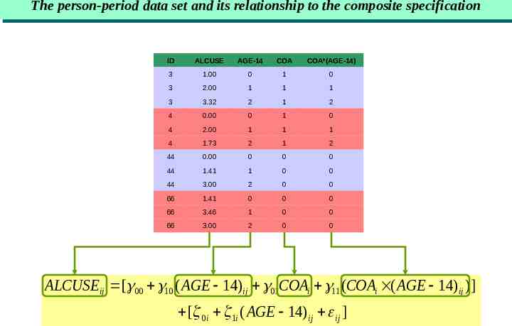
The The person-period person-period data data set set and and its its relationship relationship to to the the composite composite specification specification ID ALCUSE AGE-14 COA COA*(AGE-14) 3 1.00 0 1 0 3 2.00 1 1 1 3 3.32 2 1 2 4 0.00 0 1 0 4 2.00 1 1 1 4 1.73 2 1 2 44 0.00 0 0 0 44 1.41 1 0 0 44 3.00 2 0 0 66 1.41 0 0 0 66 3.46 1 0 0 66 3.00 2 0 0 ALCUSEij [ 00 10 ( AGE 14)ij 01COAi 11 (COAi ( AGE 14) ij )] [ 0i 1i ( AGE 14) ij ij ]
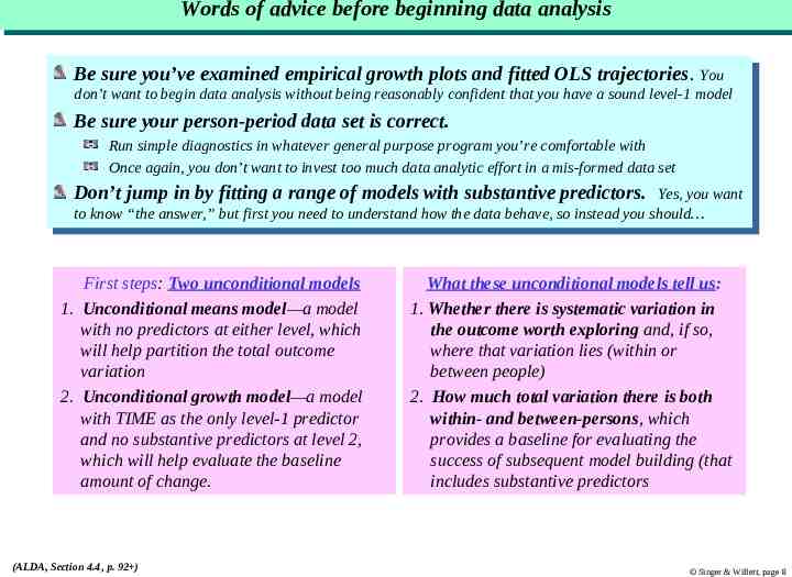
Words Words of of advice advice before before beginning beginning data data analysis analysis Be Besure sureyou’ve you’veexamined examinedempirical empiricalgrowth growthplots plotsand andfitted fittedOLS OLStrajectories. trajectories.You You don’t don’twant wanttotobegin begindata dataanalysis analysiswithout withoutbeing beingreasonably reasonablyconfident confidentthat thatyou youhave haveaasound soundlevel-1 level-1model model Be Besure sureyour yourperson-period person-perioddata dataset setisiscorrect. correct. Run Runsimple simplediagnostics diagnosticsininwhatever whatevergeneral generalpurpose purposeprogram programyou’re you’recomfortable comfortablewith with Once Onceagain, again,you youdon’t don’twant wanttotoinvest investtoo toomuch muchdata dataanalytic analyticeffort effortininaamis-formed mis-formeddata dataset set Don’t Don’tjump jumpininby byfitting fittingaarange rangeofofmodels modelswith withsubstantive substantivepredictors. predictors. Yes, Yes,you youwant want totoknow know“the “theanswer,” answer,”but butfirst firstyou youneed needtotounderstand understandhow howthe thedata databehave, behave,sosoinstead insteadyou youshould should First steps: Two unconditional models 1. Unconditional means model—a model with no predictors at either level, which will help partition the total outcome variation 2. Unconditional growth model—a model with TIME as the only level-1 predictor and no substantive predictors at level 2, which will help evaluate the baseline amount of change. (ALDA, Section 4.4, p. 92 ) What these unconditional models tell us: 1. Whether there is systematic variation in the outcome worth exploring and, if so, where that variation lies (within or between people) 2. How much total variation there is both within- and between-persons, which provides a baseline for evaluating the success of subsequent model building (that includes substantive predictors Singer & Willett, page 8
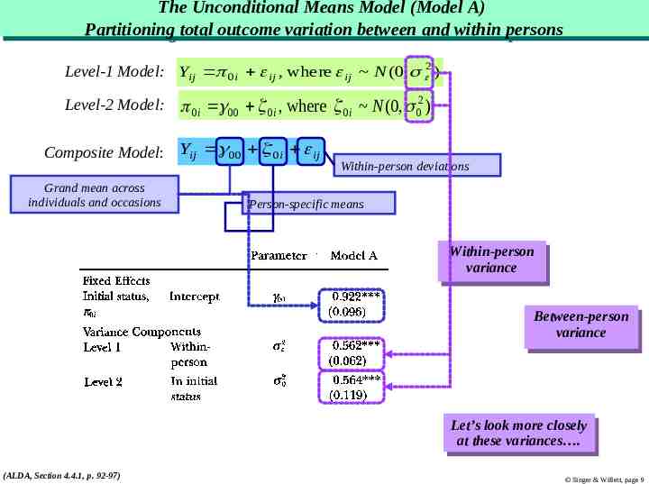
The The Unconditional Unconditional Means Means Model Model (Model (Model A) A) Partitioning Partitioning total total outcome outcome variation variation between between and and within within persons persons Level-1 Model: Yij 0i ij , where ij N (0, 2 ) Level-2 Model: 0i 00 0i , where 0i N (0, 02 ) Composite Model: Yij 00 0i ij Grand mean across individuals and occasions Within-person deviations Person-specific means Within-person Within-person variance variance Between-person Between-person variance variance Let’s Let’slook lookmore moreclosely closely at these variances . at these variances . (ALDA, Section 4.4.1, p. 92-97) Singer & Willett, page 9
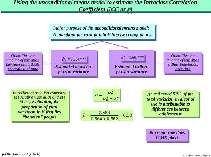
Using Using the the unconditional unconditional means means model model to to estimate estimate the the Intraclass Intraclass Correlation Correlation Coefficient Coefficient (ICC (ICC or or )) Major Majorpurpose purposeofofthe theunconditional unconditionalmeans meansmodel: model: To Topartition partitionthe thevariation variationininYYinto intotwo twocomponents components Quantifies Quantifiesthe the amount of variation amount of variation between betweenindividuals individuals regardless regardlessofoftime time ˆˆ022 00.564 .564****** 0 ˆˆ 22 00.562 .562****** Estimated Estimatedbetweenbetweenperson variance person variance Estimated Estimatedwithinwithinperson variance person variance Intraclass Intraclasscorrelation correlationcompares compares the relative magnitude the relative magnitudeofofthese these VCs by estimating the VCs by estimating the proportion proportionof oftotal total variation in Y that variation in Y thatlies lies “between” “between”people people 0022 22 00 22 0.564 ˆ 0.50 0.564 0.562 Quantifies Quantifiesthe the amount of variation amount of variation within withinindividuals individuals over overtime time An Anestimated estimated50% 50%of ofthe the total variation in alcohol total variation in alcohol use useisisattributable attributableto to differences between differences between adolescents adolescents But Butwhat whatrole roledoes does TIME play? TIME play? (ALDA, Section 4.4.1, p. 92-97) Singer & Willett, page 10
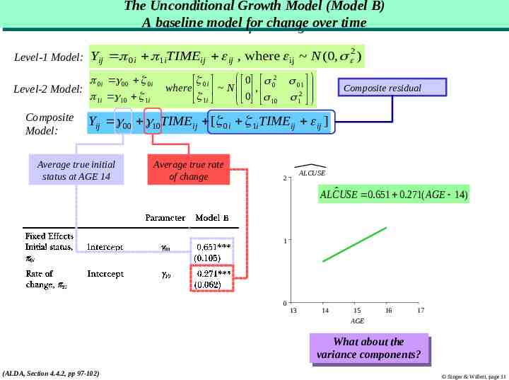
The The Unconditional Unconditional Growth Growth Model Model (Model (Model B) B) AA baseline baseline model model for for change change over over time time 2 Level-1 Model: Yij 0i 1iTIMEij ij , where ij N (0, ) 0i 00 0i Level-2 Model: 1i 10 1i Composite Model: 0 02 0i where N , 0 1i 10 01 12 Composite residual Yij 00 10TIMEij [ 0i 1iTIMEij ij ] Average true initial status at AGE 14 Average true rate of change ALCUSE 2 ALCˆ USE 0.651 0.271( AGE 14) 1 0 13 14 15 16 17 AGE What Whatabout aboutthe the variance components? variance components? (ALDA, Section 4.4.2, pp 97-102) Singer & Willett, page 11
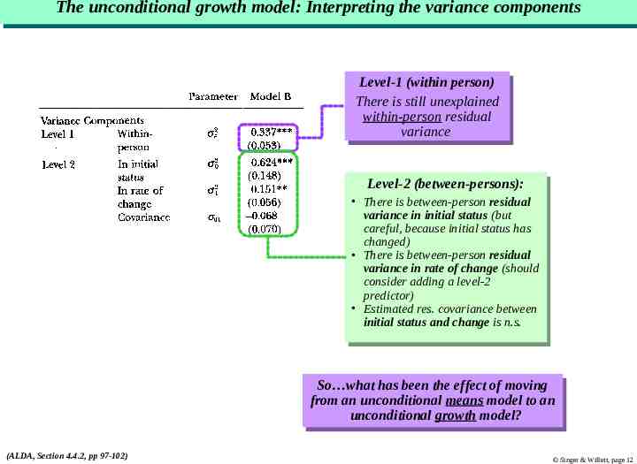
The The unconditional unconditional growth growth model: model: Interpreting Interpreting the the variance variance components components Level-1 Level-1(within (withinperson) person) There Thereisisstill stillunexplained unexplained within-person within-personresidual residual variance variance Level-2 Level-2(between-persons): (between-persons): There Thereisisbetween-person between-personresidual residual variance variancein ininitial initialstatus status(but (but careful, because initial status careful, because initial statushas has changed) changed) There Thereisisbetween-person between-personresidual residual variance in rate of change variance in rate of change(should (should consider consideradding addingaalevel-2 level-2 predictor) predictor) Estimated Estimatedres. res.covariance covariancebetween between initial status and change is initial status and change isn.s. n.s. So what So whathas hasbeen beenthe theeffect effectof ofmoving moving from an unconditional means model from an unconditional means modelto toan an unconditional growth model? unconditional growth model? (ALDA, Section 4.4.2, pp 97-102) Singer & Willett, page 12
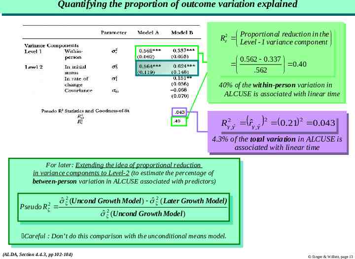
Quantifying Quantifying the the proportion proportion of of outcome outcome variation variation explained explained Proportion Proportional al reduction reductionin inthe the RR 2 2 Level variancecomponent component Level--11variance 00.562 562 00.337 337 0.40 0.40 . 562 .562 40% 40% of of the the within-person within-person variation variation in in ALCUSE ALCUSE isis associated associated with with linear linear time time 2 2 2 0.043 RRY22,Yˆˆ rˆrYˆ ,Yˆˆ 2 00.21 21 0.043 Y ,Y Y ,Y 4.3% 4.3%of ofthe thetotal totalvariation variationin inALCUSE ALCUSEisis associated associatedwith withlinear lineartime time For Forlater: later:Extending Extendingthe theidea ideaofofproportional proportionalreduction reduction ininvariance components to Level-2 (to estimate the percentage variance components to Level-2 (to estimate the percentageofof between-person between-personvariation variationininALCUSE ALCUSEassociated associatedwith withpredictors) predictors) 2 2 2(Uncond Growth Model ) ˆ 2( Later Growth Model) ˆ ˆ ˆ 2 (Uncond Growth Model ) ( Later Growth Model) Pseudo PseudoRR 2 ˆ ˆ 2 2(Uncond Growth Model ) (Uncond Growth Model ) Careful Careful: :Don’t Don’tdo dothis thiscomparison comparisonwith withthe theunconditional unconditionalmeans meansmodel. model. (ALDA, Section 4.4.3, pp 102-104) Singer & Willett, page 13
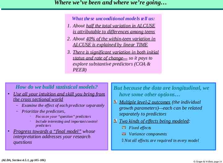
Where Where we’ve we’ve been been and and where where we’re we’re going going What these unconditional models tell us: 1. About half the total variation in ALCUSE is attributable to differences among teens 2. About 40% of the within-teen variation in ALCUSE is explained by linear TIME 3. There is significant variation in both initial status and rate of change— so it pays to explore substantive predictors (COA & PEER) How do we build statistical models? Use all your intuition and skill you bring from the cross sectional world – – Examine the effect of each predictor separately Prioritize the predictors, Focus on your “question” predictors Include interesting and important control predictors Progress towards a “final model” whose interpretation addresses your research questions (ALDA, Section 4.5.1, pp 105-106) But because the data are longitudinal, we have some other options Multiple level-2 outcomes (the individual growth parameters)—each can be related separately to predictors Two kinds of effects being modeled: Fixed effects Variance components Not all effects are required in every model Singer & Willett, page 14
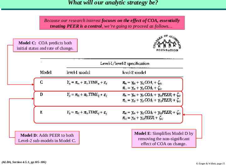
What What will will our our analytic analytic strategy strategy be? be? Because our research interest focuses on the effect of COA, essentially treating PEER is a control, we’re going to proceed as follows Model C: COA predicts both initial status and rate of change. Model D: Adds PEER to both Level-2 sub-models in Model C. (ALDA, Section 4.5.1, pp 105-106) Model E: Simplifies Model D by removing the non-significant effect of COA on change. Singer & Willett, page 15
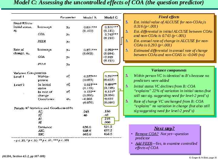
Model Model C: C: Assessing Assessing the the uncontrolled uncontrolled effects effects of of COA COA (the (the question question predictor) predictor) Fixed Fixedeffects effects Est. initial value of ALCUSE Est. initial value of ALCUSEfor fornon-COAs non-COAsisis 0.316 (p .001) 0.316 (p .001) Est. Est.differential differentialinininitial initialALCUSE ALCUSEbetween betweenCOAs COAs and andnon-COAs non-COAsisis0.743 0.743(p .001) (p .001) Est. Est.annual annualrate rateofofchange changeininALCUSE ALCUSEfor fornonnonCOAs COAsisis0.293 0.293(p .001) (p .001) Estimated Estimateddifferential differentialininannual annualrate rateofofchange change between COAs and non-COAS is –0.049 between COAs and non-COAS is –0.049(ns) (ns) Variance Variancecomponents components Within person VC is identical Within person VC is identicaltotoB’s B’sbecause becauseno no predictors were added predictors were added Initial Initialstatus statusVC VCdeclines declinesfrom fromB:B:COA COA “explains” 22% of variation in initial “explains” 22% of variation in initialstatus status(but (but still stat sig. suggesting need for level-2 pred’s) still stat sig. suggesting need for level-2 pred’s) Rate Rateofofchange changeVC VCunchanged unchangedfrom fromB:B:COA COA “explains” no variation in change (but also “explains” no variation in change (but alsostill still sig suggesting need for level-2 pred’s) sig suggesting need for level-2 pred’s) Next Nextstep? step? Remove RemoveCOA? COA? Not Notyet—question yet—question predictor predictor Add AddPEER—Yes, PEER—Yes,totoexamine examinecontrolled controlled effects of COA effects of COA (ALDA, Section 4.5.2, pp 107-108) Singer & Willett, page 16
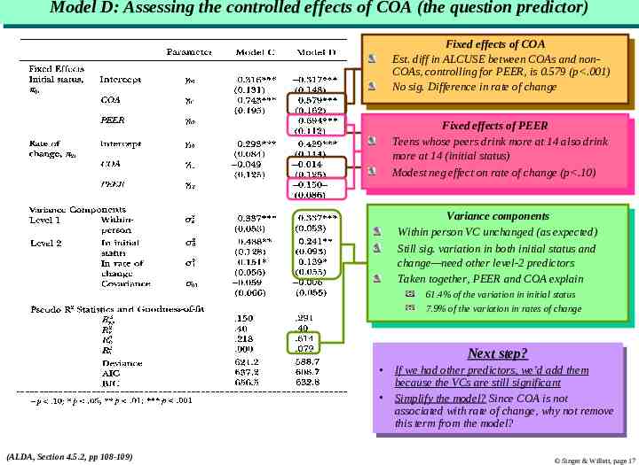
Model Model D: D: Assessing Assessing the the controlled controlled effects effects of of COA COA (the (the question question predictor) predictor) Fixed Fixedeffects effectsofofCOA COA Est. diff in ALCUSE between Est. diff in ALCUSE betweenCOAs COAsand andnonnonCOAs, COAs,controlling controllingfor forPEER, PEER,isis0.579 0.579(p .001) (p .001) No Nosig. sig.Difference Differenceininrate rateofofchange change Fixed Fixedeffects effectsofofPEER PEER Teens whose peers drink more Teens whose peers drink moreatat14 14also alsodrink drink more at 14 (initial status) more at 14 (initial status) Modest Modestneg negeffect effecton onrate rateofofchange change(p .10) (p .10) Variance Variancecomponents components Within person VC unchanged Within person VC unchanged(as (asexpected) expected) Still Stillsig. sig.variation variationininboth bothinitial initialstatus statusand and change—need other level-2 predictors change—need other level-2 predictors Taken Takentogether, together,PEER PEERand andCOA COAexplain explain 61.4% of the variation in initial status 61.4% of the variation in initial status 7.9% of the variation in rates of change 7.9% of the variation in rates of change Next Nextstep? step? IfIfwe wehad hadother otherpredictors, predictors,we’d we’dadd addthem them because the VCs are still significant because the VCs are still significant Simplify Simplifythe themodel? model?Since SinceCOA COAisisnot not associated with rate of change, associated with rate of change,why whynot notremove remove this term from the model? this term from the model? (ALDA, Section 4.5.2, pp 108-109) Singer & Willett, page 17
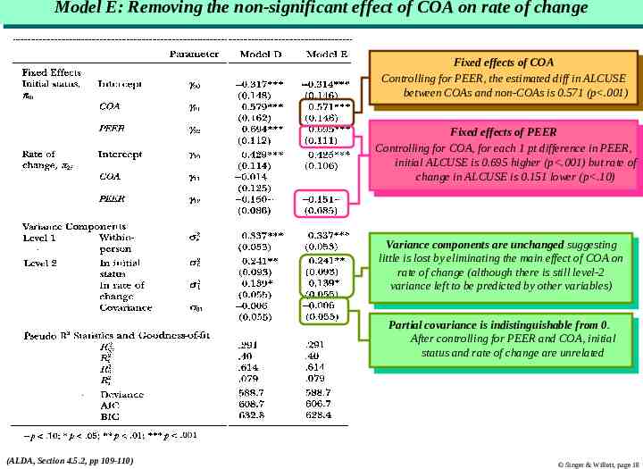
Model Model E: E: Removing Removing the the non-significant non-significant effect effect of of COA COA on on rate rate of of change change Fixed Fixedeffects effectsofofCOA COA Controlling for PEER, the estimated Controlling for PEER, the estimateddiff diffininALCUSE ALCUSE between COAs and non-COAs is 0.571 (p .001) between COAs and non-COAs is 0.571 (p .001) Fixed Fixedeffects effectsofofPEER PEER Controlling for COA, for each 1 pt Controlling for COA, for each 1 ptdifference differenceininPEER, PEER, initial ALCUSE is 0.695 higher (p .001) but rate initial ALCUSE is 0.695 higher (p .001) but rateofof change changeininALCUSE ALCUSEisis0.151 0.151lower lower(p .10) (p .10) Variance Variancecomponents componentsare areunchanged unchangedsuggesting suggesting little is lost by eliminating the main effect little is lost by eliminating the main effectofofCOA COAon on rate of change (although there is still level-2 rate of change (although there is still level-2 variance varianceleft lefttotobebepredicted predictedbybyother othervariables) variables) Partial Partialcovariance covarianceisisindistinguishable indistinguishablefrom from0.0. After Aftercontrolling controllingfor forPEER PEERand andCOA, COA,initial initial status statusand andrate rateofofchange changeare areunrelated unrelated (ALDA, Section 4.5.2, pp 109-110) Singer & Willett, page 18
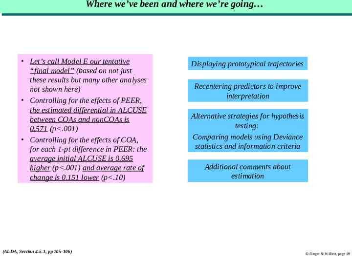
Where Where we’ve we’ve been been and and where where we’re we’re going going Let’s call Model E our tentative “final model” (based on not just these results but many other analyses not shown here) Controlling for the effects of PEER, the estimated differential in ALCUSE between COAs and nonCOAs is 0.571 (p .001) Controlling for the effects of COA, for each 1-pt difference in PEER: the average initial ALCUSE is 0.695 higher (p .001) and average rate of change is 0.151 lower (p .10) (ALDA, Section 4.5.1, pp 105-106) Displaying prototypical trajectories Recentering predictors to improve interpretation Alternative strategies for hypothesis testing: Comparing models using Deviance statistics and information criteria Additional comments about estimation Singer & Willett, page 19
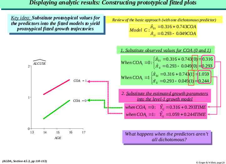
Displaying Displaying analytic analytic results: results: Constructing Constructing prototypical prototypical fitted fitted plots plots Key Keyidea: idea:Substitute Substituteprototypical prototypicalvalues valuesfor for the predictors into the fitted models to yield the predictors into the fitted models to yield prototypical prototypicalfitted fittedgrowth growthtrajectories trajectories Review of the basic approach (with one dichotomous predictor) Model C : ˆ 0i 0.316 0.743COA ˆ1i 0.293 0.049COA 1. Substitute observed values for COA (0 and 1) 2 ALCUSE COA 1 1 COA 0 ˆ 0.316 0.743(0) 0.316 When COAi 0 : 0i ˆ1i 0.293 0.049(0) 0.293 ˆ 0i 0.316 0.743(1) 1.059 When COAi 1 ˆ 1i 0.293 0.049(1) 0.244 2. Substitute the estimated growth parameters into the level-1 growth model when COA 0 : Yˆ 0.316 0.293TIME i ij when COAi 1 : Yˆij 1.059 0.244TIME 0 13 14 15 AGE (ALDA, Section 4.5.3, pp 110-113) 16 17 What Whathappens happenswhen whenthe thepredictors predictorsaren’t aren’t all dichotomous? all dichotomous? Singer & Willett, page 20
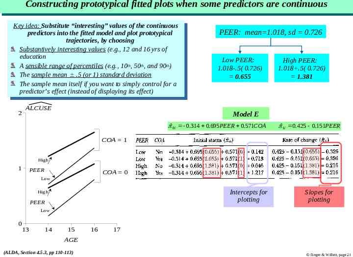
Constructing Constructing prototypical prototypical fitted fitted plots plots when when some some predictors predictors are are continuous continuous Key Keyidea: idea:Substitute Substitute“interesting” “interesting”values valuesofofthe thecontinuous continuous predictors into the fitted model and plot prototypical predictors into the fitted model and plot prototypical trajectories, trajectories,by bychoosing choosing Substantively interesting values (e.g., Substantively interesting values (e.g.,12 12and and16 16yrs yrsofof education education th th th AAsensible sensiblerange rangeofofpercentiles percentiles(e.g., (e.g.,10 10th, ,50 50th, ,and and90 90th) ) The Thesample samplemean mean .5.5(or (or1)1)standard standarddeviation deviation The sample mean itself if you want to simply The sample mean itself if you want to simplycontrol controlfor foraa predictor’s predictor’seffect effect(instead (insteadofofdisplaying displayingits itseffect) effect) 2 ALCUSE PEER: mean 1.018, sd 0.726 Low PEER: 1.018-.5( 0.726) 0.655 High PEER: 1.018 .5( 0.726) 1.381 Model E ˆ 0i 0.314 0.695PEER 0.571COA ˆ1i 0.425 0.151PEER COA 1 High 1 PEER COA 0 Low Intercepts for plotting High PEER Slopes for plotting Low 0 13 14 15 16 17 AGE (ALDA, Section 4.5.3, pp 110-113) Singer & Willett, page 21
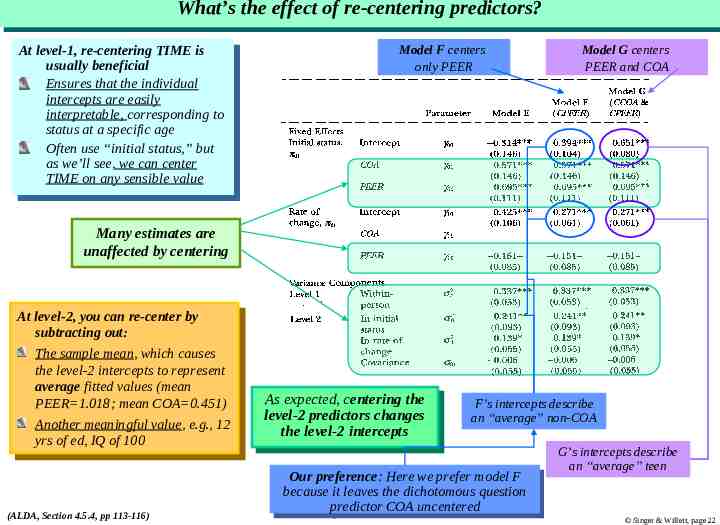
What’s What’s the the effect effect of of re-centering re-centering predictors? predictors? At Atlevel-1, level-1,re-centering re-centeringTIME TIMEisis usually usuallybeneficial beneficial Ensures that Ensures thatthe theindividual individual intercepts are easily intercepts are easily interpretable, interpretable,corresponding correspondingtoto status statusatataaspecific specificage age Often use “initial status,” Often use “initial status,”but but asaswe’ll see, we can center we’ll see, we can center TIME TIMEon onany anysensible sensiblevalue value Model F centers only PEER Model G centers PEER and COA Many estimates are unaffected by centering At Atlevel-2, level-2,you youcan canre-center re-centerby by subtracting out: subtracting out: The Thesample samplemean, mean,which whichcauses causes the level-2 intercepts to represent the level-2 intercepts to represent average averagefitted fittedvalues values(mean (mean PEER 1.018; mean COA 0.451) PEER 1.018; mean COA 0.451) Another Anothermeaningful meaningfulvalue, value,e.g., e.g.,12 12 yrs of ed, IQ of 100 yrs of ed, IQ of 100 (ALDA, Section 4.5.4, pp 113-116) As Asexpected, expected,centering centeringthe the level-2 predictors changes level-2 predictors changes the thelevel-2 level-2intercepts intercepts F’s intercepts describe an “average” non-COA Our Ourpreference: preference:Here Herewe weprefer prefermodel modelFF because becauseititleaves leavesthe thedichotomous dichotomousquestion question predictor COA uncentered predictor COA uncentered G’s intercepts describe an “average” teen Singer & Willett, page 22
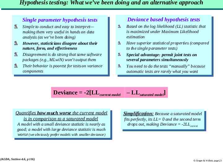
Hypothesis Hypothesis testing: testing: What What we’ve we’ve been been doing doing and and an an alternative alternative approach approach Single Singleparameter parameterhypothesis hypothesistests tests Simple Simpletotoconduct conductand andeasy easytotointerpret— interpret— making them very useful in hands making them very useful in handson ondata data analysis (as we’ve been doing) analysis (as we’ve been doing) However, However,statisticians statisticiansdisagree disagreeabout abouttheir their nature, form, and effectiveness nature, form, and effectiveness Disagreement Disagreementisisdo dostrong strongthat thatsome somesoftware software packages (e.g., MLwiN) won’t output them packages (e.g., MLwiN) won’t output them Their Theirbehavior behaviorisispoorest poorestfor fortests testson onvariance variance components components Deviance -2[LLcurrent model Quantifies Quantifieshow howmuch muchworse worsethe thecurrent currentmodel model isisinincomparison to a saturated model comparison to a saturated model AAmodel modelwith withaasmall smalldeviance deviancestatistic statisticisisnearly nearlyasas good; good;aamodel modelwith withlarge largedeviance deviancestatistic statisticisismuch much worse (we obviously prefer models with smaller deviance) worse (we obviously prefer models with smaller deviance) (ALDA, Section 4.6, p 116) Deviance Deviancebased basedhypothesis hypothesistests tests Based Basedon onthe thelog loglikelihood likelihood(LL) (LL)statistic statisticthat that isismaximized under Maximum Likelihood maximized under Maximum Likelihood estimation estimation Have Havesuperior superiorstatistical statisticalproperties properties(compared (compared totothe single parameter tests) the single parameter tests) Special Specialadvantage: advantage:permit permitjoint jointtests testson on several parameters simultaneously several parameters simultaneously You Youneed needtotodo dothe thetests tests“manually” “manually”because because automatic tests are rarely what you want automatic tests are rarely what you want – LLsaturated model] Simplification: Simplification:Because Becauseaasaturated saturatedmodel model fits fitsperfectly, perfectly,its itsLL LL 00and andthe thesecond secondterm term drops out, making Deviance -2LL drops out, making Deviance -2LLcurrent current Singer & Willett, page 23
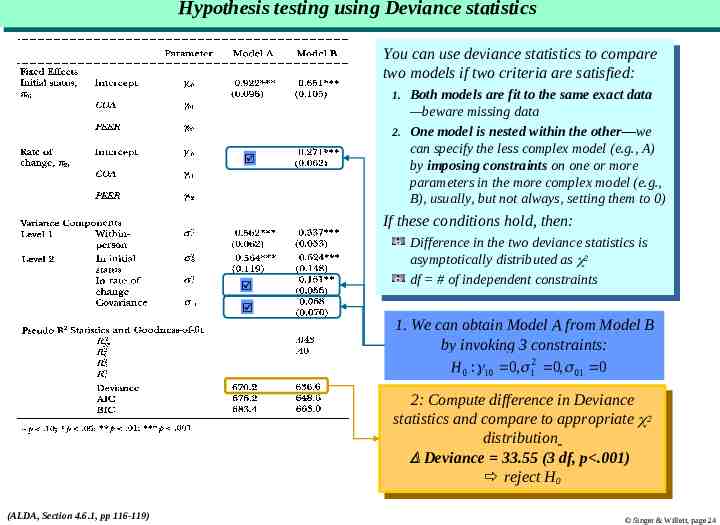
Hypothesis Hypothesis testing testing using using Deviance Deviance statistics statistics You Youcan canuse usedeviance deviancestatistics statisticstotocompare compare two models if two criteria are satisfied: two models if two criteria are satisfied: 1. Both models are fit to the same exact data 1. Both models are fit to the same exact data —beware —bewaremissing missingdata data 2. One model is nested within the other—we 2. One model is nested within the other—we can canspecify specifythe theless lesscomplex complexmodel model(e.g., (e.g.,A) A) by imposing constraints on one or more by imposing constraints on one or more parameters parametersininthe themore morecomplex complexmodel model(e.g., (e.g., B), usually, but not always, setting them to B), usually, but not always, setting them to0)0) IfIfthese theseconditions conditionshold, hold,then: then: Difference Differenceininthe thetwo twodeviance deviancestatistics statisticsisis 2 asymptotically asymptoticallydistributed distributedasas 2 dfdf ##ofofindependent independentconstraints constraints 1. We can obtain Model A from Model B by invoking 3 constraints: H 0 : 10 0, 12 0, 01 0 2:2:Compute Computedifference differenceininDeviance Deviance 2 statistics and compare to appropriate statistics and compare to appropriate 2 distribution distribution Deviance Deviance 33.55 33.55(3(3df, df,p .001) p .001) reject rejectHH0 0 (ALDA, Section 4.6.1, pp 116-119) Singer & Willett, page 24
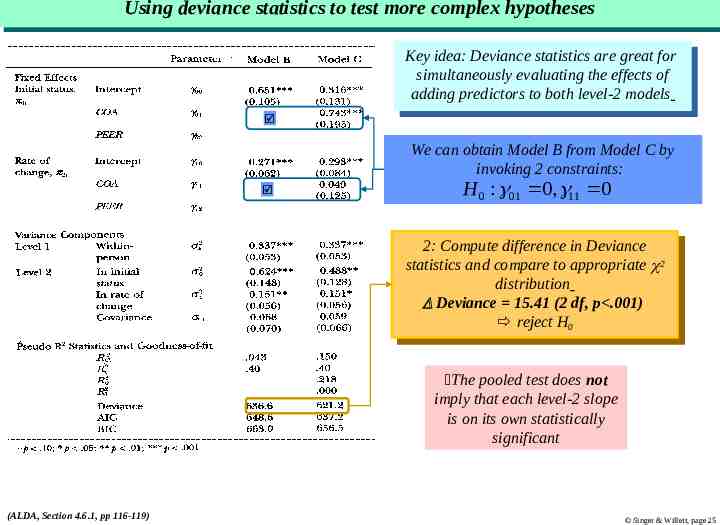
Using Using deviance deviance statistics statistics to to test test more more complex complex hypotheses hypotheses Key Keyidea: idea:Deviance Deviancestatistics statisticsare aregreat greatfor for simultaneously evaluating the effects of simultaneously evaluating the effects of adding addingpredictors predictorstotoboth bothlevel-2 level-2models models We can obtain Model B from Model C by invoking 2 constraints: H 0 : 01 0, 11 0 2:2:Compute Computedifference differenceininDeviance Deviance 2 statistics statisticsand andcompare comparetotoappropriate appropriate 2 distribution distribution Deviance Deviance 15.41 15.41(2(2df, df,p .001) p .001) reject H reject H0 0 The pooled test does not imply that each level-2 slope is on its own statistically significant (ALDA, Section 4.6.1, pp 116-119) Singer & Willett, page 25
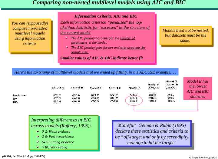
Comparing Comparing non-nested non-nested multilevel multilevel models models using using AIC AIC and and BIC BIC You Youcan can(supposedly) (supposedly) compare comparenon-nested non-nested multilevel multilevelmodels models using information using information criteria criteria Information InformationCriteria: Criteria:AIC AICand andBIC BIC Each Eachinformation informationcriterion criterion“penalizes” “penalizes”the thelogloglikelihood statistic for “excesses” in the structure likelihood statistic for “excesses” in the structureofof the thecurrent currentmodel model The TheAIC AICpenalty penaltyaccounts accountsfor forthe thenumber numberofof parameters in the model. parameters in the model. The BIC penalty goes further and also accounts for The BIC penalty goes further and also accounts for sample size. sample size. Models Modelsneed neednot notbe benested, nested, but datasets must be but datasets must bethe the same. same. Smaller Smallervalues valuesofofAIC AIC&&BIC BICindicate indicatebetter betterfitfit Here’s the taxonomy of multilevel models that we ended up fitting, in the ALCUSE example . Model E has the lowest AIC and BIC statistics Interpreting Interpretingdifferences differencesin inBIC BIC across acrossmodels models(Raftery, (Raftery,1995): 1995): 0-2: 0-2:Weak Weakevidence evidence 2-6: Positive 2-6: Positiveevidence evidence 6-10: Strong evidence 6-10: Strong evidence 10: 10:Very Verystrong strong (ALDA, Section 4.6.4, pp 120-122) Careful: Gelman & Rubin (1995) Careful: Gelman & Rubin (1995) declare these statistics and criteria to declare these statistics and criteria to be “off-target and only by serendipity be “off-target and only by serendipity manage to hit the target” manage to hit the target” Singer & Willett, page 26
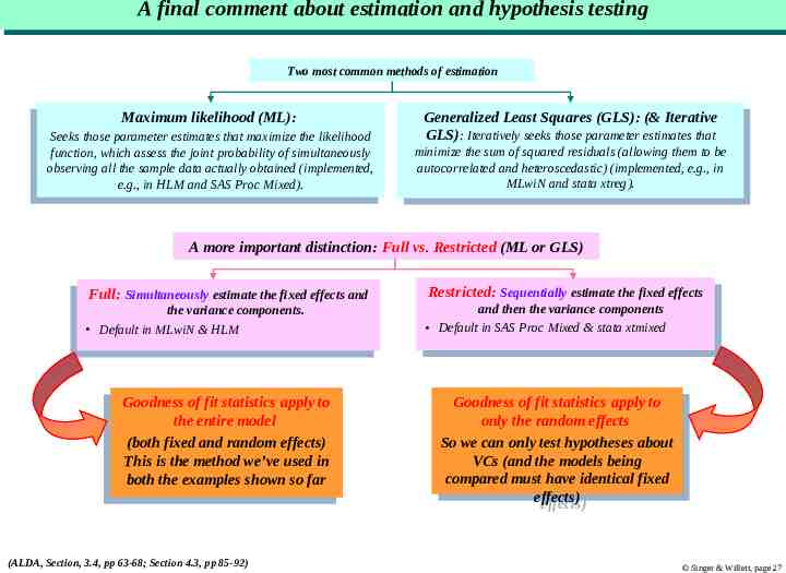
AA final final comment comment about about estimation estimation and and hypothesis hypothesis testing testing Two most common methods of estimation Maximumlikelihood likelihood(ML): (ML): Maximum Seeks those parameter estimates that maximize the likelihood Seeks those parameter estimates that maximize the likelihood function, which assess the joint probability of simultaneously function, which assess the joint probability of simultaneously observingall allthe thesample sampledata dataactually actuallyobtained obtained(implemented, (implemented, observing e.g., in HLM and SAS Proc Mixed). e.g., in HLM and SAS Proc Mixed). Generalized GeneralizedLeast LeastSquares Squares(GLS): (GLS):(& (&Iterative Iterative GLS) : Iteratively seeks those parameter estimates that GLS): Iteratively seeks those parameter estimates that minimize the sum of squared residuals (allowing them to be minimize the sum of squared residuals (allowing them to be autocorrelated and heteroscedastic) (implemented, e.g., in autocorrelated and heteroscedastic) (implemented, e.g., in MLwiN and stata xtreg). MLwiN and stata xtreg). A more important distinction: Full vs. Restricted (ML or GLS) Full:Simultaneously Simultaneouslyestimate estimatethe thefixed fixedeffects effectsand and Full: the variance components. the variance components. Default in MLwiN & HLM Default in MLwiN & HLM Goodnessofoffitfitstatistics statisticsapply applytoto Goodness theentire entiremodel model the (bothfixed fixedand andrandom randomeffects) effects) (both Thisisisthe themethod methodwe’ve we’veused usedinin This boththe theexamples examplesshown shownsosofar far both (ALDA, Section, 3.4, pp 63-68; Section 4.3, pp 85-92) Restricted: Restricted:Sequentially Sequentiallyestimate estimatethe thefixed fixedeffects effects and then the variance components and then the variance components Default in SAS Proc Mixed & stata xtmixed Default in SAS Proc Mixed & stata xtmixed Goodness Goodnessofoffitfitstatistics statisticsapply applytoto only onlythe therandom randomeffects effects So Sowe wecan canonly onlytest testhypotheses hypothesesabout about VCs (and the models being VCs (and the models being compared comparedmust musthave haveidentical identicalfixed fixed effects) effects) Singer & Willett, page 27
Other Other topics topics covered covered in in Chapter Chapter Four Four Using UsingWald Waldstatistics statisticstototest testcomposite compositehypotheses hypotheses about fixed effects (§4.7)—generalization about fixed effects (§4.7)—generalizationofofthe the “parameter estimate divided by its standard error” “parameter estimate divided by its standard error” approach approachthat thatallows allowsyou youtototest testcomposite compositehypotheses hypotheses about fixed effects, even if you’ve used restricted about fixed effects, even if you’ve used restricted estimation estimationmethods methods Evaluating Evaluatingthe thetenability tenabilityofofthe themodel’s model’sassumptions assumptions (§4.8) (§4.8) Checking Checkingfunctional functionalform form Checking Checkingnormality normality Checking Checkinghomoscedasticity homoscedasticity Model-Based Model-Based(empirical (empiricalBayes) Bayes)estimates estimatesofofthe the individual growth parameters (§4.9) Superior individual growth parameters (§4.9) Superiorestimates estimates that combine OLS estimates with population average that combine OLS estimates with population average estimates estimatesthat thatare areusually usuallyyour yourbest bestbet betififyou youwould wouldlike like totodisplay individual growth trajectories for particular display individual growth trajectories for particular sample samplemembers members Singer & Willett, page 28