Data and Computer Communications Tenth Edition by William Stallings


54 Slides2.65 MB
Data and Computer Communications Tenth Edition by William Stallings Data and Computer Communications, Tenth Edition by William Stallings, (c) Pearson Education - 2013
CHAPTER 19 Routing
Routing in Switched Data Networks "I tell you," went on Syme with passion, "that every time a train comes in I feel that it has broken past batteries of besiegers, and that man has won a battle against chaos. You say contemptuously that when one has left Sloane Square one must come to Victoria. I say that one might do a thousand things instead, and that whenever I really come there I have the sense of hairbreadth escape. And when I hear the guard shout out the word 'Victoria', it is not an unmeaning word. It is to me the cry of a herald announcing conquest. It is to me indeed 'Victoria'; it is the victory of Adam." —The Man Who Was Thursday, G.K. Chesterton
Routing in Packet Switching Networks Key design issue for (packet) switched networks Select route across network between end nodes Characteristics required: Correctness Simplicity Robustness Stability Fairness Optimality Efficiency
Table 19.1 Elements of Routing Techniques for Packet-Switching Networks PerformanceCriteria Number of hops Cost Delay Throughput Decision Time Packet (datagram) Session (virtual circuit) Decision Place Each node (distributed) Central node (centralized) Originating node (source) Network Information Source None Local Adjacent node Nodes along route All nodes Network Information UpdateTiming Continuous Periodic Major load change Topology change
Performance Criteria Used for selection of route Simplest is to choose “minimum hop” Can be generalized as “least cost” routing Because “least cost” is more flexible it is more common than “minimum hop”
8 5 3 N2 N3 6 5 8 2 3 N1 2 2 3 3 1 1 2 4 1 7 N6 N4 1 1 N5 Figure19.1 ExampleNetwork Configuration
Decision Time and Place Decision time Packet or virtual circuit basis Fixed or dynamically changing Decision place Distributed - made by each node More complex, but more robust Centralized – made by a designated node Source – made by source station
Network Information Source and Update Timing Routing decisions usually based on knowledge of network, traffic load, and link cost Distributed routing Using local knowledge, information from adjacent nodes, information from all nodes on a potential route Central routing Collect information from all nodes Issue of update timing Depends on routing strategy Fixed - never updated Adaptive - regular updates
Routing Strategies - Fixed Routing Use a single permanent route for each source to destination pair of nodes Determined using a least cost algorithm Route is fixed Until a change in network topology Based on expected traffic or capacity Advantage is simplicity Disadvantage is lack of flexibility Does not react to network failure or congestion
CENTRAL ROUTING DIRECTORY From Node To Node 1 2 3 4 5 6 1 — 1 5 2 4 5 2 2 — 5 2 4 5 3 4 3 — 5 3 5 4 4 4 5 — 4 5 5 4 4 5 5 — 5 6 4 4 5 5 6 — Node 1 Directory Node2 Directory Node3 Directory Destination Next Node Destination Next Node Destination Next Node 2 2 1 1 1 5 3 4 3 3 2 5 4 4 4 4 4 5 5 4 5 4 5 5 6 4 6 4 6 5 Node 4 Directory Node5 Directory Node6 Directory Destination Next Node Destination Next Node Destination Next Node 1 2 1 4 1 5 2 2 2 4 2 5 3 5 3 3 3 5 5 5 4 4 4 5 6 5 6 6 5 5 Figure19.2 Fixed Routing (using Figure 19.1)
Routing Strategies - Flooding Packet sent by node to every neighbor Eventually multiple copies arrive at destination No network information required Each packet is uniquely numbered so duplicates can be discarded Need to limit incessant retransmission of packets Nodes can remember identity of packets retransmitted Can include a hop count in packets
2 3 3 6 1 3 3 4 5 (a) First hop 2 3 2 2 2 2 2 2 2 1 6 2 2 4 5 (b) Second hop 1 1 1 1 3 1 1 1 1 1 1 2 1 1 1 4 1 1 1 1 1 6 1 1 1 1 1 5 (c) Third hop Figure19.3 FloodingExample(hop count 3)
Properties of Flooding All possible routes are tried Highly robust Can be used to send emergency messages At least one packet will have taken minimum hop route Nodes directly or indirectly connected to source are visited Disadvantages: High traffic load generated Security concerns
Routing Strategies - Random Routing Simplicity of flooding with much less traffic load Node selects one outgoing path for retransmission of incoming packet Selection can be random or round robin A refinement is to select outgoing path based on probability calculation No network information needed Random route is typically neither least cost nor minimum hop
Routing Strategies - Adaptive Routing Used by almost all packet switching networks Routing decisions change as conditions on the network change due to failure or congestion Requires information about network Disadvantages: Decisions more complex Tradeoff between quality of network information and overhead Reacting too quickly can cause oscillation Reacting too slowly means information may be irrelevant
Adaptive Routing Advantages Improved performance Aid in congestion control These benefits depend on the soundness of the design and nature of the load
Classification of Adaptive Routing Strategies A convenient way to classify is on the basis of information source Local (isolated) Route to outgoing link with shortest queue Can include bias for each destination Rarely used - does not make use of available information Adjacent nodes Takes advantage of delay and outage information Distributed or centralized All nodes Like adjacent
To 2 Node 4's Bias Table for Destination 6 Next Node Bias 1 9 2 6 3 3 5 0 To 3 To 1 Node4 Figure19.4 Exampleof Isolated AdaptiveRouting To 5
ARPANET Routing Strategies 1st Generation Distance Vector Routing 1969 Distributed adaptive using estimated delay Queue length used as estimate of delay Version of Bellman-Ford algorithm Node exchanges delay vector with neighbors Update routing table based on incoming information Doesn't consider line speed, just queue length and responds slowly to congestion
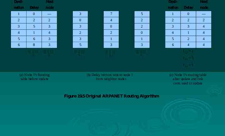
Desti- Next Desti- Next nation Delay node nation Delay node 1 0 — 3 7 5 1 0 — 2 2 2 0 4 2 2 2 2 3 5 3 3 0 2 3 3 4 4 1 4 2 2 0 4 1 4 5 6 3 3 1 1 5 2 4 6 8 3 5 3 3 6 4 4 D1 S1 D 2 D 3 D 4 I 1,2 2 I 1,3 5 I 1,4 1 (a) Node 1's Routing table before update (b) Delay vectors sent to node 1 from neighbor nodes Figure19.5 Original ARPANET Routing Algorithm (c) Node 1's routing table after update and link costs used in update
5 3 N2 N3 5 N6 2 2 N1 9 1 2 1 N4 9 N5 Figure19.6 Network for Exampleof Figure19.5a
ARPANET Routing Strategies 2nd Generation Link-State Routing 1979 Distributed adaptive using delay criterion Using timestamps of arrival, departure and ACK times Re-computes average delays every 10 seconds Any changes are flooded to all other nodes Re-computes routing using Dijkstra’s algorithm Good under light and medium loads Under heavy loads, little correlation between reported delays and those experienced
A B Figure19.7 Packet-SwitchingNetwork Subject to Oscillations
ARPANET Routing Strategies 3rd Generation 1987 Link cost calculation changed Damp routing oscillations Reduce routing overhead Measure average delay over last 10 seconds and transform into link utilization estimate Normalize this based on current value and previous results Set link cost as function of average utilization
5 Theoretical queueing delay Delay (hops) 4 3 Metric for satellitelink 2 Metric for terrestrial link 1 0 0 0.1 0.2 0.3 0.4 0.5 0.6 0.7 Estimated utilization Figure19.8 ARPANET Delay Metrics 0.8 0.9 1.0
Internet Routing Protocols Routers are responsible for receiving and forwarding packets through the interconnected set of networks Makes routing decisions based on knowledge of the topology and traffic/delay conditions of the internet Routers exchange routing information using a special routing protocol Two Routing information concepts in considering the routing function: Information about the topology and delays of the internet Routing algorithm The algorithm used to make a routing decision for a particular datagram, based on current routing information
Autonomous Systems (AS) Exhibits the following characteristics: Is a set of routers and networks managed by a single organization Consists of a group of routers exchanging information via a common routing protocol Except in times of failure, is connected (in a graph-theoretic sense); there is a path between any pair of nodes
Interior Router Protocol (IRP) A shared routing protocol which passes routing information between routers within an AS Custom tailored to specific applications and requirements
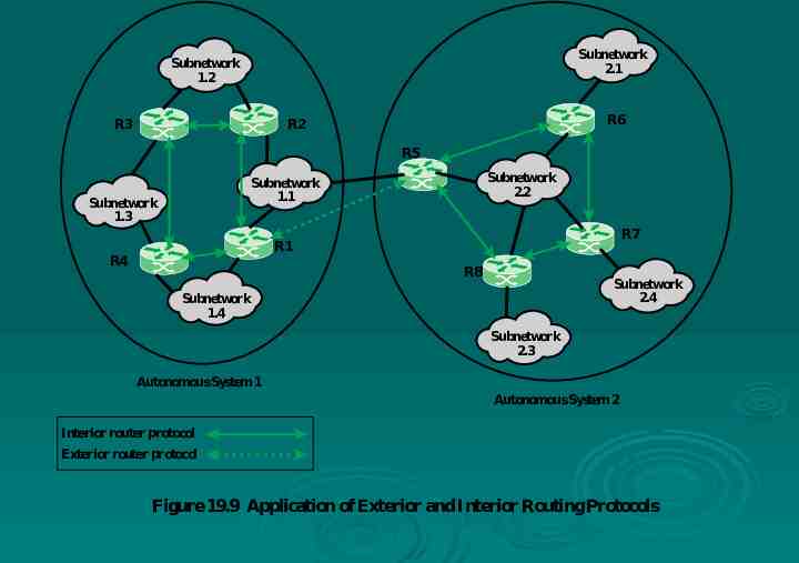
Subnetwork 2.1 Subnetwork 1.2 R6 R2 R3 R5 Subnetwork 2.2 Subnetwork 1.1 Subnetwork 1.3 R7 R1 R4 R8 Subnetwork 2.4 Subnetwork 1.4 Subnetwork 2.3 Autonomous System 1 Autonomous System 2 Interior router protocol Exterior router protocol Figure19.9 Application of Exterior and Interior Routing Protocols
Exterior Router Protocol (ERP) Protocol used to pass routing information between routers in different ASs Will need to pass less information than an IRP for the following reason: If a datagram is to be transferred from a host in one AS to a host in another AS, a router in the first system need only determine the target AS and devise a route to get into that target system Once the datagram enters the target AS, the routers within that system can cooperate to deliver the datagram The ERP is not concerned with, and does not know about, the details of the route Examples Border Gateway Protocol (BGP) Open Shortest Path First (OSPF)
Approaches to Routing Internet routing protocols employ one of three approaches to gathering and using routing information: Distance-vector routing Path-vector routing Link-state routing
Distance-Vector Routing Requires that each node exchange information with its neighboring nodes Two nodes are said to be neighbors if they are both directly connected to the same network Used in the first-generation routing algorithm for ARPANET Each node maintains a vector of link costs for each directly attached network and distance and next-hop vectors for each destination Routing Information Protocol (RIP) uses this approach
Link-State Routing Designed to overcome the drawbacks of distance-vector routing When a router is initialized, it determines the link cost on each of its network interfaces The router then advertises this set of link costs to all other routers in the internet topology, not just neighboring routers From then on, the router monitors its link costs Whenever there is a significant change the router again advertises its set of link costs to all other routers in the configuration The OSPF protocol is an example The second-generation routing algorithm for ARPANET also uses this approach
Path-Vector Routing Alternative to dispense with routing metrics and simply provide information about which networks can be reached by a given router and the Ass visited in order to reach the destination network by this route Differs from a distance-vector algorithm in two respects: The path-vector approach does not include a distance or cost estimate Each block of routing information lists all of the ASs visited in order to reach the destination network by this route
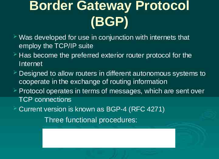
Border Gateway Protocol (BGP) Was developed for use in conjunction with internets that employ the TCP/IP suite Has become the preferred exterior router protocol for the Internet Designed to allow routers in different autonomous systems to cooperate in the exchange of routing information Protocol operates in terms of messages, which are sent over TCP connections Current version is known as BGP-4 (RFC 4271) Three functional procedures: Neighbor acquisition Neighbor reachability Network reachability
Table 19.2 BGP-4 Messages Open Used to open a neighbor relationship with another router. Update Used to (1) transmit information about a single route and/or (2) list multiple routes to be withdrawn. Keepalive Used to (1) acknowledge an Open message and (2) periodically confirm the neighbor relationship. Notification Send when an error condition is detected.
Neighbor Acquisition Occurs when two neighboring routers in different autonomous systems agree to exchange routing information regularly Two routers send Open messages to each other after a TCP connection is established If each router accepts the request, it returns a Keepalive message in response Protocol does not address the issue of how one router knows the address or even the existence of another router nor how it decides that it needs to exchange routing information with that particular router
Octets Octets 16 Marker 16 Marker 2 Length 2 Length 1 1 Type Version 1 Type 2 2 My Autonomous System UnfeasibleRoutes Length 2 Hold Time variable Withdrawn Routes 2 Total Path Attributes Length 4 BGP Identifier variable Path Attributes variable Network Layer Reachability Information 1 Opt Parameter Length variable Optional Parameters (a) Open Message (b) UpdateMessage Octets Octets 16 Marker 16 Marker 2 Length 2 Length 1 Type 1 1 1 Type Error Code Error Subcode (c) KeepaliveMessage variable Data (d) Notification Message Figure19.10 BGP MessageFormats
Open Shortest Path First (OSPF) Protocol RFC 2328 Used as the interior router protocol in TCP/IP networks Computes a route through the internet that incurs the least cost based on a userconfigurable metric of cost Is able to equalize loads over multiple equal-cost paths
N12 N1 3 R1 1 1 N2 1 3 R3 8 8 8 6 N12 R6 6 7 2 R7 N4 1 9 N11 N15 5 1 R10 3 N6 3 R9 1 R11 1 1 2 N7 1 2 10 R8 N8 4 N9 H1 R5 6 6 2 R2 8 7 1 N14 8 8 R4 N3 N13 N10 R12 Figure19.11 A SampleAutonomous System
N12 N1 N13 R1 3 8 1 8 N3 1 8 1 R3 3 R2 N11 7 R6 6 N4 R5 7 6 8 2 8 8 R4 1 N2 6 N12 6 2 R7 5 9 7 3 R9 3 1 R11 1 1 R10 N9 N14 N6 1 2 R8 N8 1 N15 4 1 H1 10 2 N10 N7 R12 Figure19.12 Directed Graph of Autonomous System of Figure19.11
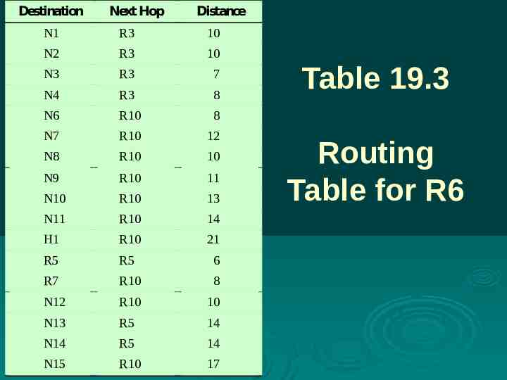
Destination Next Hop Distance N1 R3 10 N2 R3 10 N3 R3 7 N4 R3 8 N6 R10 8 N7 R10 12 N8 R10 10 N9 R10 11 N10 R10 13 N11 R10 14 H1 R10 21 R5 R5 6 R7 R10 8 N12 R10 10 N13 R5 14 N14 R5 14 N15 R10 17 Table 19.3 Routing Table for R6
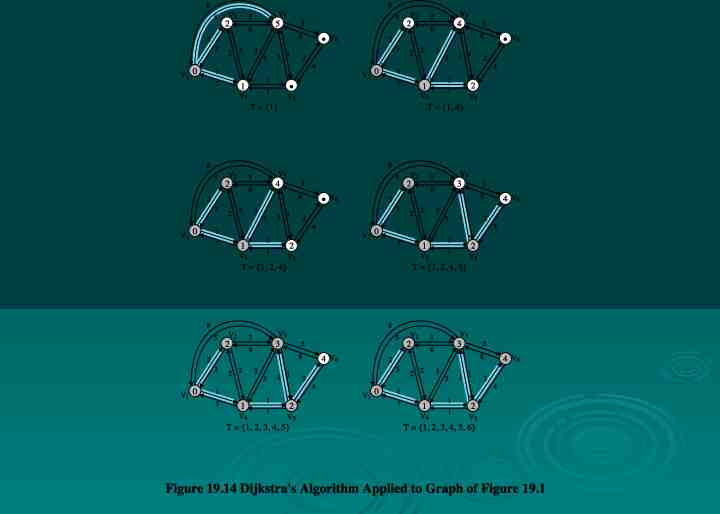
Dijkstra’s Algorithm Finds shortest paths from given source nodesto all other nodes Develop paths in order of increasing path length Algorithm runs in stages Each time adding node with next shortest path Algorithm terminates when all nodes have been added to T
Dijkstra’s Algorithm Method Step 1 [Initialization] T {s} Set of nodes so far incorporated L(n) w(s, n) for n s Initial path costs to neighboring nodes are simply link costs Step 2 [Get Next Node]Also incorporate the edge that is Find neighboring node not in T with least-cost path from s Incorporate node into T incident on that node and a node in T that contributes to the path Step 3 [Update Least-Cost Paths] L(n) min[L(n), L(x) w(x, n)] for all n Ï T If latter term is minimum, path from s to n is path from s to x concatenated with edge from x to n
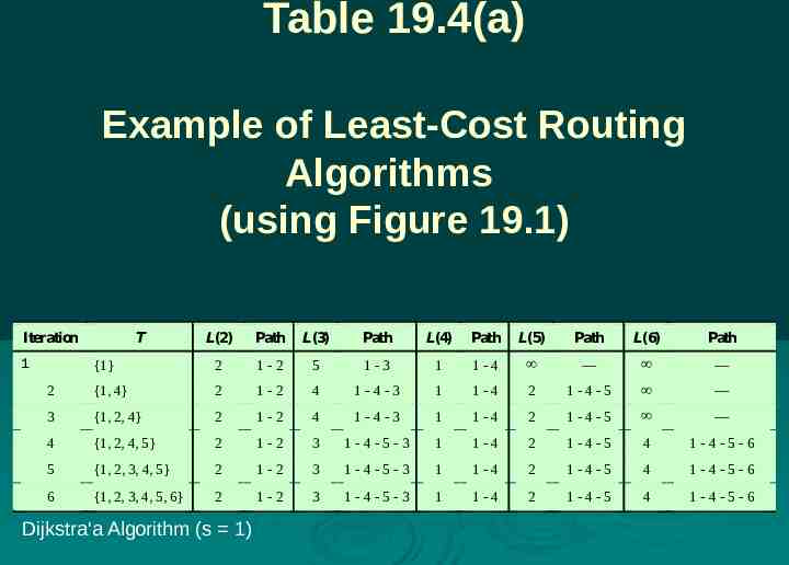
Table 19.4(a) Example of Least-Cost Routing Algorithms (using Figure 19.1) Iteration L(2) Path L(3) Path L(4) Path L(5) Path L(6) Path {1} 2 1-2 5 1-3 1 1-4 — — 2 {1, 4} 2 1-2 4 1-4-3 1 1-4 2 1-4-5 — 3 {1, 2, 4} 2 1-2 4 1-4-3 1 1-4 2 1-4-5 — 4 {1, 2, 4, 5} 2 1-2 3 1-4-5-3 1 1-4 2 1-4-5 4 1-4-5-6 5 {1, 2, 3, 4, 5} 2 1-2 3 1-4-5-3 1 1-4 2 1-4-5 4 1-4-5-6 6 {1, 2, 3, 4, 5, 6} 2 1-2 3 1-4-5-3 1 1-4 2 1-4-5 4 1-4-5-6 1 T Dijkstra'a Algorithm (s 1)
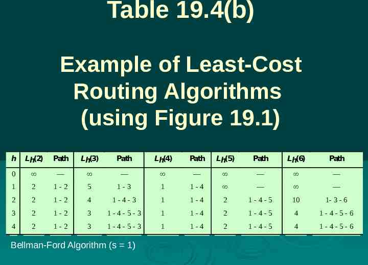
Bellman-Ford Algorithm Find shortest paths from given node subject to constraint that paths contain at most one link Findthe shortest paths with a constraint of paths of at most two links Proceeds in stages
Bellman-Ford Algorithm Step1 [Initialization] L0(n) , for all n s Lh(s) 0, for all h Step 2 [Update] For each successive h 0 For each n s, compute: Lh 1(n) minj[Lh(j) w(j,n)] Connect n with predecessor node j that gives min Eliminate any connection of n with different predecessor node formed during an earlier iteration Path from s to n terminates with link from j to n
Table 19.4(b) Example of Least-Cost Routing Algorithms (using Figure 19.1) h Lh(2) Path Lh(3) Path Lh(4) Path Lh(5) Path Lh(6) Path 0 — — — — — 1 2 1-2 5 1-3 1 1-4 — — 2 2 1-2 4 1-4-3 1 1-4 2 1-4-5 10 1- 3 - 6 3 2 1-2 3 1-4-5-3 1 1-4 2 1-4-5 4 1-4-5-6 4 2 1-2 3 1-4-5-3 1 1-4 2 1-4-5 4 1-4-5-6 Bellman-Ford Algorithm (s 1)
Comparison Bellman-Ford Calculation for node n needs link cost to neighboring nodes plus total cost to each neighbor from s Each node can maintain set of costs and paths for every other node Can exchange information with direct neighbors Can update costs and paths based on information from neighbors and knowledge of link costs Dijkstra Each node needs complete topology Must know link costs of all links in network Must exchange information with all other nodes
Evaluation Dependent on Processing time of algorithms Amount of information required from other nodes Implementation specific If link costs depend on traffic, which depends on routes chosen, may have feedback instability Both converge under static topology and costs If link costs change, algorithms attempt to catch up Both converge to same solution
Summary Routing in packetswitching networks Characteristics Routing strategies Examples: Routing in ARPANET First generation: Distance Vector Routing Second generation: Link-State Routing Third generation Internet routing protocols Autonomous systems Approaches to routing Border gateway protocol OSPF protocol Least-cost algorithms Dijkstra’s algorithm Bellman-Ford algorithm Comparison