CS267 Lecture 2 Single Processor Machines: Memory Hierarchies and

77 Slides1.73 MB
CS267 Lecture 2 Single Processor Machines: Memory Hierarchies and Processor Features Case Study: Tuning Matrix Multiply James Demmel http://www.cs.berkeley.edu/ demmel/cs267 Spr16/ 1
Rough List of Topics Basics of computer architecture, memory hierarchies, performance Parallel Programming Models and Machines Shared Memory and Multithreading Distributed Memory and Message Passing Data parallelism, GPUs Cloud computing Parallel languages and libraries Shared memory threads and OpenMP MPI Other Languages , frameworks (UPC, CUDA, Spark, PETSC, “Pattern Language”, ) “Seven Dwarfs” of Scientific Computing Dense & Sparse Linear Algebra Structured and Unstructured Grids Spectral methods (FFTs) and Particle Methods 6 additional motifs Graph algorithms, Graphical models, Dynamic Programming, Branch & Bound, FSM, Logic General techniques Autotuning, Load balancing, performance tools Applications: climate modeling, materials science, astrophysics (guest lecturers) 01/21/2016 CS267 - Lecture 2 2
Motivation Most applications run at 10% of the “peak” performance of a system Peak is the maximum the hardware can physically execute Much of this performance is lost on a single processor, i.e., the code running on one processor often runs at only 1020% of the processor peak Most of the single processor performance loss is in the memory system Moving data takes much longer than arithmetic and logic To understand this, we need to look under the hood of modern processors For today, we will look at only a single “core” processor These issues will exist on processors within any parallel computer 01/21/2016 CS267 - Lecture 2 3
Possible conclusions to draw from today’s lecture “Computer architectures are fascinating, and I really want to understand why apparently simple programs can behave in such complex ways!” “I want to learn how to design algorithms that run really fast no matter how complicated the underlying computer architecture.” “I hope that most of the time I can use fast software that someone else has written and hidden all these details from me so I don’t have to worry about them!” All of the above, at different points in time 01/21/2016 CS267 - Lecture 2 4
Outline Idealized and actual costs in modern processors Memory hierarchies Use of microbenchmarks to characterized performance Parallelism within single processors Case study: Matrix Multiplication Use of performance models to understand performance Attainable lower bounds on communication 01/21/2016 CS267 - Lecture 2 5
Outline Idealized and actual costs in modern processors Memory hierarchies Use of microbenchmarks to characterized performance Parallelism within single processors Case study: Matrix Multiplication Use of performance models to understand performance Attainable lower bounds on communication 01/21/2016 CS267 - Lecture 2 6
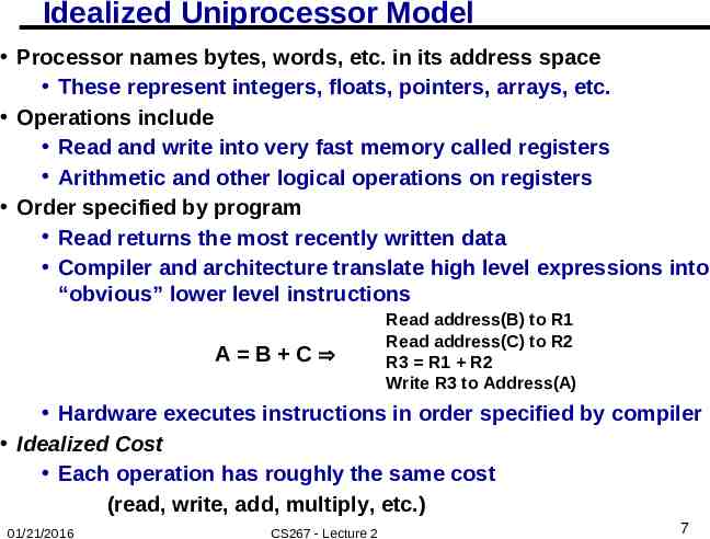
Idealized Uniprocessor Model Processor names bytes, words, etc. in its address space These represent integers, floats, pointers, arrays, etc. Operations include Read and write into very fast memory called registers Arithmetic and other logical operations on registers Order specified by program Read returns the most recently written data Compiler and architecture translate high level expressions into “obvious” lower level instructions A B C Read address(B) to R1 Read address(C) to R2 R3 R1 R2 Write R3 to Address(A) Hardware executes instructions in order specified by compiler Idealized Cost Each operation has roughly the same cost (read, write, add, multiply, etc.) 01/21/2016 CS267 - Lecture 2 7
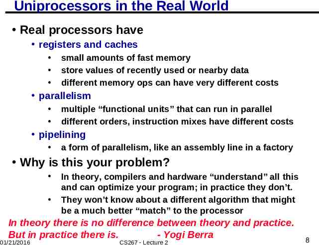
Uniprocessors in the Real World Real processors have registers and caches small amounts of fast memory store values of recently used or nearby data different memory ops can have very different costs parallelism multiple “functional units” that can run in parallel different orders, instruction mixes have different costs pipelining a form of parallelism, like an assembly line in a factory Why is this your problem? In theory, compilers and hardware “understand” all this and can optimize your program; in practice they don’t. They won’t know about a different algorithm that might be a much better “match” to the processor In theory there is no difference between theory and practice. But in practice there is. - Yogi Berra 01/21/2016 CS267 - Lecture 2 8
Outline Idealized and actual costs in modern processors Memory hierarchies Temporal and spatial locality Basics of caches Use of microbenchmarks to characterized performance Parallelism within single processors Case study: Matrix Multiplication Use of performance models to understand performance Attainable lower bounds on communication 01/21/2016 CS267 - Lecture 2 9
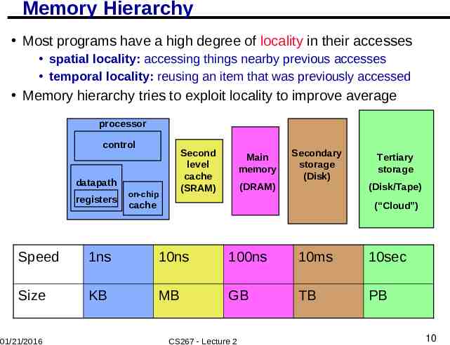
Memory Hierarchy Most programs have a high degree of locality in their accesses spatial locality: accessing things nearby previous accesses temporal locality: reusing an item that was previously accessed Memory hierarchy tries to exploit locality to improve average processor control Second level cache (SRAM) datapath registers on-chip Main memory (DRAM) Secondary storage (Disk) cache Tertiary storage (Disk/Tape) (“Cloud”) Speed 1ns 10ns 100ns 10ms 10sec Size KB MB GB TB PB 01/21/2016 CS267 - Lecture 2 10
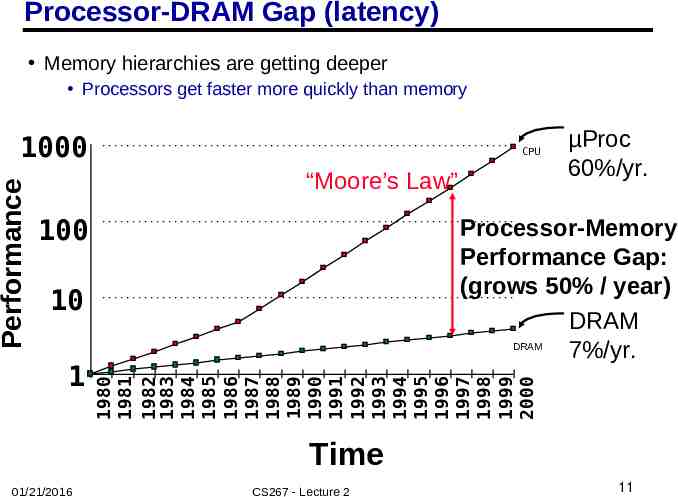
Processor-DRAM Gap (latency) Memory hierarchies are getting deeper Processors get faster more quickly than memory CPU “Moore’s Law” 100 Processor-Memory Performance Gap: (grows 50% / year) DRAM DRAM 7%/yr. 10 1 µProc 60%/yr. 1980 1981 1982 1983 1984 1985 1986 1987 1988 1989 1990 1991 1992 1993 1994 1995 1996 1997 1998 1999 2000 Performance 1000 Time 01/21/2016 CS267 - Lecture 2 11
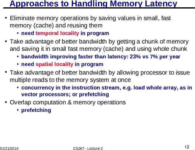
Approaches to Handling Memory Latency Eliminate memory operations by saving values in small, fast memory (cache) and reusing them need temporal locality in program Take advantage of better bandwidth by getting a chunk of memory and saving it in small fast memory (cache) and using whole chunk bandwidth improving faster than latency: 23% vs 7% per year need spatial locality in program Take advantage of better bandwidth by allowing processor to issue multiple reads to the memory system at once concurrency in the instruction stream, e.g. load whole array, as in vector processors; or prefetching Overlap computation & memory operations prefetching 01/21/2016 CS267 - Lecture 2 12
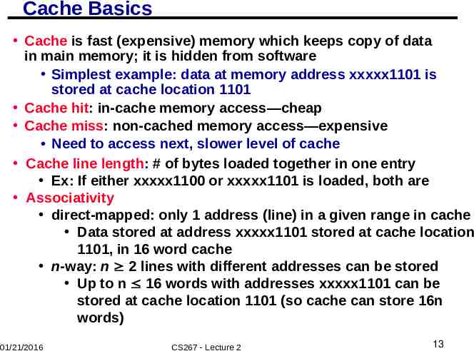
Cache Basics Cache is fast (expensive) memory which keeps copy of data in main memory; it is hidden from software Simplest example: data at memory address xxxxx1101 is stored at cache location 1101 Cache hit: in-cache memory access—cheap Cache miss: non-cached memory access—expensive Need to access next, slower level of cache Cache line length: # of bytes loaded together in one entry Ex: If either xxxxx1100 or xxxxx1101 is loaded, both are Associativity direct-mapped: only 1 address (line) in a given range in cache Data stored at address xxxxx1101 stored at cache location 1101, in 16 word cache n-way: n 2 lines with different addresses can be stored Up to n 16 words with addresses xxxxx1101 can be stored at cache location 1101 (so cache can store 16n words) 01/21/2016 CS267 - Lecture 2 13
Why Have Multiple Levels of Cache? On-chip vs. off-chip On-chip caches are faster, but limited in size A large cache has delays Hardware to check longer addresses in cache takes more time Associativity, which gives a more general set of data in cache, also takes more time Some examples: Cray T3E eliminated one cache to speed up misses IBM uses a level of cache as a “victim cache” which is cheaper There are other levels of the memory hierarchy Register, pages (TLB, virtual memory), And it isn’t always a hierarchy 01/21/2016 CS267 - Lecture 2 14
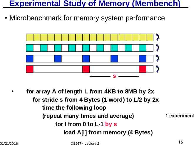
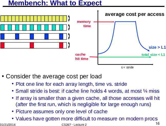
Experimental Study of Memory (Membench) Microbenchmark for memory system performance s 01/21/2016 for array A of length L from 4KB to 8MB by 2x for time stride s from 4 Bytes (1 word) to L/2 by 2x the following loop time themany following (repeat timesloop and average) (repeat and average) for imany from times 0 to L-1 forload i from to L-1memory by s A[i]0 from (4 Bytes) load A[i] from memory (4 Bytes) CS267 - Lecture 2 1 experiment 15
Membench: What to Expect average cost per access memory time size L1 cache hit time total size L1 s stride Consider the average cost per load Plot one line for each array length, time vs. stride Small stride is best: if cache line holds 4 words, at most ¼ miss If array is smaller than a given cache, all those accesses will hit (after the first run, which is negligible for large enough runs) Picture assumes only one level of cache Values have gotten more difficult to measure on modern procs 01/21/2016 CS267 - Lecture 2 16
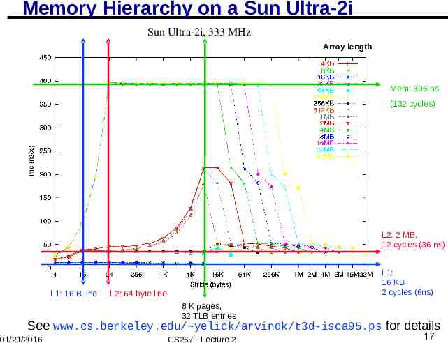
Memory Hierarchy on a Sun Ultra-2i Sun Ultra-2i, 333 MHz Array length Mem: 396 ns (132 cycles) L2: 2 MB, 12 cycles (36 ns) L1: 16 B line L1: 16 KB 2 cycles (6ns) L2: 64 byte line 8 K pages, 32 TLB entries See www.cs.berkeley.edu/ yelick/arvindk/t3d-isca95.ps for details 01/21/2016 CS267 - Lecture 2 17
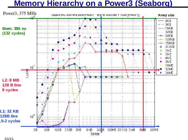
Memory Hierarchy on a Power3 (Seaborg) Power3, 375 MHz Array size Mem: 396 ns (132 cycles) L2: 8 MB 128 B line 9 cycles L1: 32 KB 128B line .5-2 cycles 01/21/2016 CS267 - Lecture 2 18
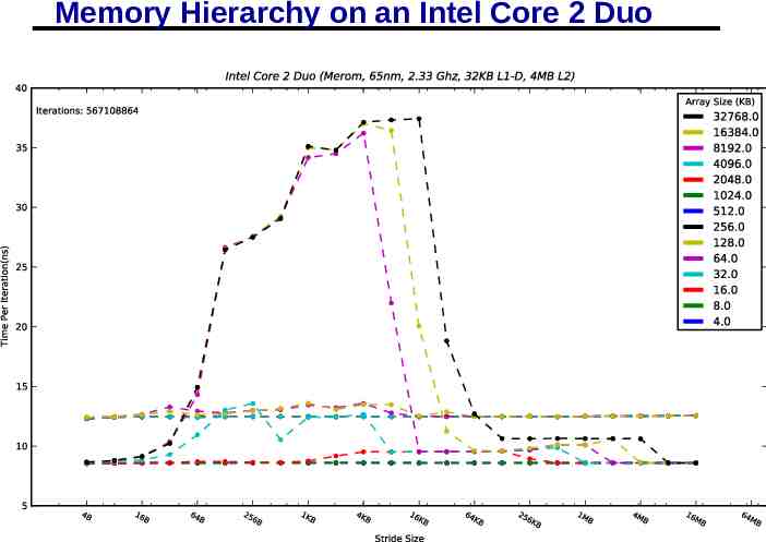
Memory Hierarchy on an Intel Core 2 Duo 01/21/2016 CS267 - Lecture 2 19
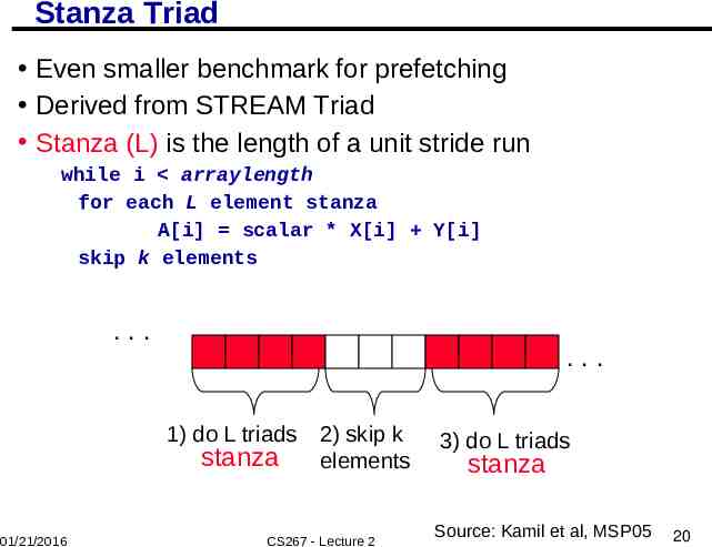
Stanza Triad Even smaller benchmark for prefetching Derived from STREAM Triad Stanza (L) is the length of a unit stride run while i arraylength for each L element stanza A[i] scalar * X[i] Y[i] skip k elements . . 1) do L triads stanza 01/21/2016 2) skip k elements CS267 - Lecture 2 3) do L triads stanza Source: Kamil et al, MSP05 20
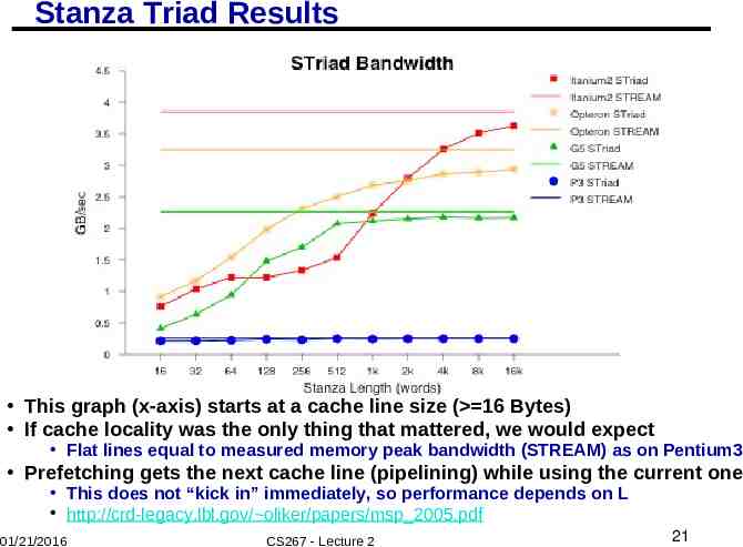
Stanza Triad Results This graph (x-axis) starts at a cache line size ( 16 Bytes) If cache locality was the only thing that mattered, we would expect Flat lines equal to measured memory peak bandwidth (STREAM) as on Pentium3 Prefetching gets the next cache line (pipelining) while using the current one This does not “kick in” immediately, so performance depends on L http://crd-legacy.lbl.gov/ oliker/papers/msp 2005.pdf 01/21/2016 CS267 - Lecture 2 21
Lessons Actual performance of a simple program can be a complicated function of the architecture Slight changes in the architecture or program change the performance significantly To write fast programs, need to consider architecture True on sequential or parallel processor We would like simple models to help us design efficient algorithms We will illustrate with a common technique for improving cache performance, called blocking or tiling Idea: used divide-and-conquer to define a problem that fits in register/L1-cache/L2-cache 01/21/2016 CS267 - Lecture 2 22
Outline Idealized and actual costs in modern processors Memory hierarchies Use of microbenchmarks to characterized performance Parallelism within single processors Hidden from software (sort of) Pipelining SIMD units Case study: Matrix Multiplication Use of performance models to understand performance Attainable lower bounds on communication 01/21/2016 CS267 - Lecture 2 23
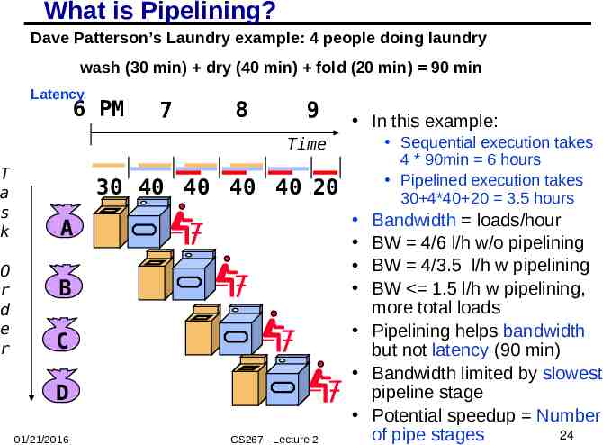
What is Pipelining? Dave Patterson’s Laundry example: 4 people doing laundry wash (30 min) dry (40 min) fold (20 min) 90 min Latency 6 PM 7 8 9 In this example: Sequential execution takes 4 * 90min 6 hours Pipelined execution takes 30 4*40 20 3.5 hours Time T a s k O r d e r 30 40 40 40 40 20 A B C D 01/21/2016 CS267 - Lecture 2 Bandwidth loads/hour BW 4/6 l/h w/o pipelining BW 4/3.5 l/h w pipelining BW 1.5 l/h w pipelining, more total loads Pipelining helps bandwidth but not latency (90 min) Bandwidth limited by slowest pipeline stage Potential speedup Number 24 of pipe stages
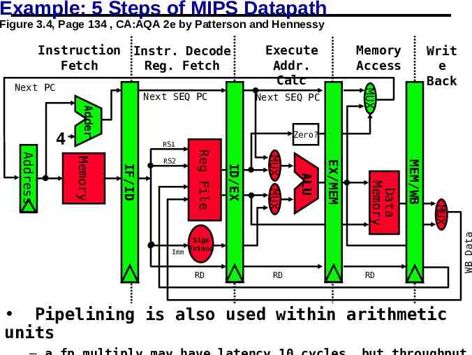
Example: 5 Steps of MIPS Datapath Figure 3.4, Page 134 , CA:AQA 2e by Patterson and Hennessy Instruction Instr. Decode Fetch Reg. Fetch Next SEQ PC Next SEQ PC Adder Writ e Back Zero? RS1 MUX MEM/WB Data Memory EX/MEM MUX ALU MUX ID/EX Imm Reg File IF/ID Memory Address RS2 Sign Extend RD RD RD Pipelining is also used within arithmetic 25 units 01/21/2016 CS267 - Lecture 2 WB Data 4 Memory Access MUX Next PC Execute Addr. Calc
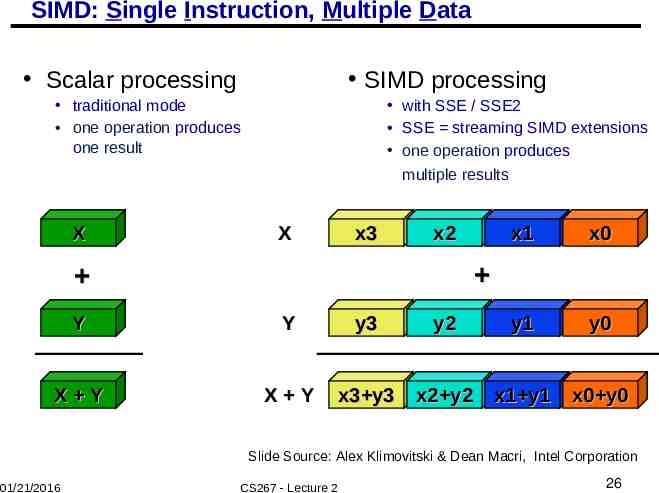
SIMD: Single Instruction, Multiple Data Scalar processing SIMD processing traditional mode one operation produces one result X with SSE / SSE2 SSE streaming SIMD extensions one operation produces multiple results X x3 x2 x1 x0 Y Y y3 y2 y1 y0 X Y X Y x3 y3 x2 y2 x1 y1 x0 y0 Slide Source: Alex Klimovitski & Dean Macri, Intel Corporation 01/21/2016 CS267 - Lecture 2 26
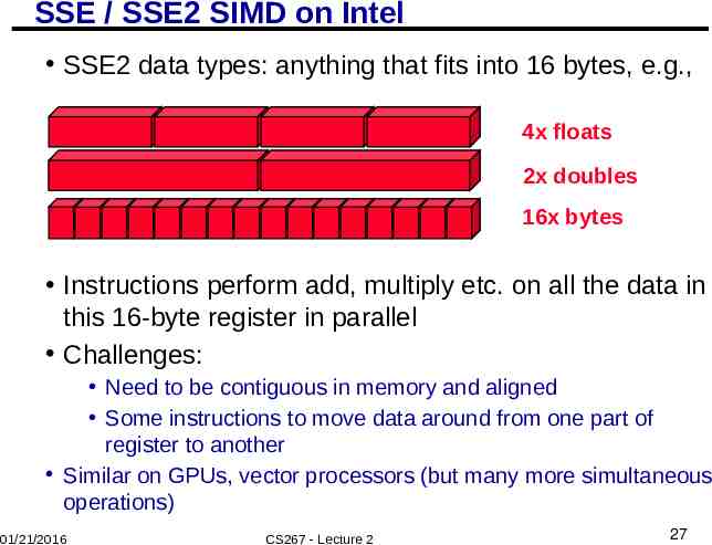
SSE / SSE2 SIMD on Intel SSE2 data types: anything that fits into 16 bytes, e.g., 4x floats 2x doubles 16x bytes Instructions perform add, multiply etc. on all the data in this 16-byte register in parallel Challenges: Need to be contiguous in memory and aligned Some instructions to move data around from one part of register to another Similar on GPUs, vector processors (but many more simultaneous operations) 01/21/2016 CS267 - Lecture 2 27
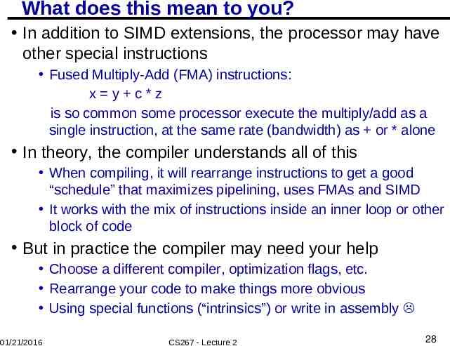
What does this mean to you? In addition to SIMD extensions, the processor may have other special instructions Fused Multiply-Add (FMA) instructions: x y c*z is so common some processor execute the multiply/add as a single instruction, at the same rate (bandwidth) as or * alone In theory, the compiler understands all of this When compiling, it will rearrange instructions to get a good “schedule” that maximizes pipelining, uses FMAs and SIMD It works with the mix of instructions inside an inner loop or other block of code But in practice the compiler may need your help Choose a different compiler, optimization flags, etc. Rearrange your code to make things more obvious Using special functions (“intrinsics”) or write in assembly 01/21/2016 CS267 - Lecture 2 28
Outline Idealized and actual costs in modern processors Memory hierarchies Use of microbenchmarks to characterized performance Parallelism within single processors Case study: Matrix Multiplication Use of performance models to understand performance Attainable lower bounds on communication Simple cache model Warm-up: Matrix-vector multiplication Naïve vs optimized Matrix-Matrix Multiply Minimizing data movement Beating O(n3) operations Practical optimizations (continued next time) 01/21/2016 CS267 - Lecture 2 29
Why Matrix Multiplication? An important kernel in many problems Appears in many linear algebra algorithms Bottleneck for dense linear algebra, including Top500 One of the 7 dwarfs / 13 motifs of parallel computing Closely related to other algorithms, e.g., transitive closure on a graph using Floyd-Warshall Optimization ideas can be used in other problems The best case for optimization payoffs The most-studied algorithm in high performance computing 01/21/2016 CS267 - Lecture 2 30
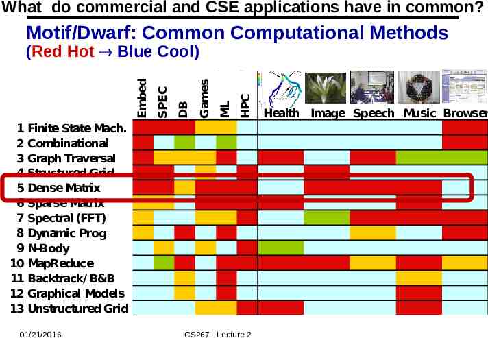
What do commercial and CSE applications have in common? Motif/Dwarf: Common Computational Methods HPC ML Games DB SPEC Embed (Red Hot Blue Cool) 1 Finite State Mach. 2 Combinational 3 Graph Traversal 4 Structured Grid 5 Dense Matrix 6 Sparse Matrix 7 Spectral (FFT) 8 Dynamic Prog 9 N-Body 10 MapReduce 11 Backtrack/ B&B 12 Graphical Models 13 Unstructured Grid 01/21/2016 CS267 - Lecture 2 Health Image Speech Music Browser
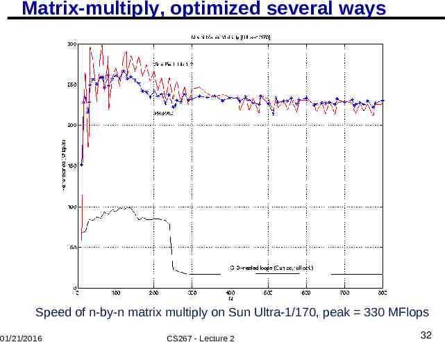
Matrix-multiply, optimized several ways Speed of n-by-n matrix multiply on Sun Ultra-1/170, peak 330 MFlops 01/21/2016 CS267 - Lecture 2 32
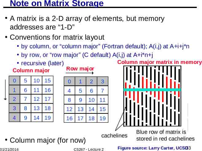
Note on Matrix Storage A matrix is a 2-D array of elements, but memory addresses are “1-D” Conventions for matrix layout by column, or “column major” (Fortran default); A(i,j) at A i j*n by row, or “row major” (C default) A(i,j) at A i*n j Column major matrix in memory recursive (later) Column major Row major 0 5 10 15 0 1 2 3 1 6 11 16 4 5 6 7 2 7 12 17 8 9 10 11 3 8 13 18 12 13 14 15 4 9 14 19 16 17 18 19 Column major (for now) 01/21/2016 cachelines CS267 - Lecture 2 Blue row of matrix is stored in red cachelines Figure source: Larry Carter, UCSD33
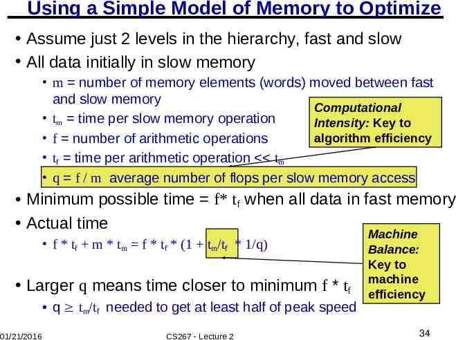
Using a Simple Model of Memory to Optimize Assume just 2 levels in the hierarchy, fast and slow All data initially in slow memory m number of memory elements (words) moved between fast and slow memory Computational tm time per slow memory operation Intensity: Key to algorithm efficiency f number of arithmetic operations tf time per arithmetic operation tm q f / m average number of flops per slow memory access Minimum possible time f* tf when all data in fast memory Actual time f * tf m * tm f * tf * (1 tm/tf * 1/q) Larger q means time closer to minimum f * tf q tm/tf needed to get at least half of peak speed 01/21/2016 CS267 - Lecture 2 Machine Balance: Key to machine efficiency 34
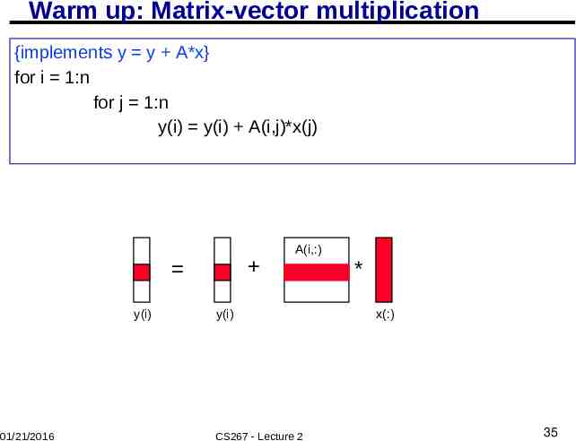
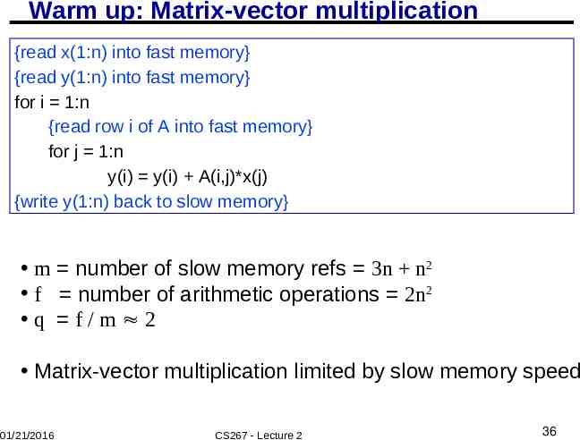
Warm up: Matrix-vector multiplication {implements y y A*x} for i 1:n for j 1:n y(i) y(i) A(i,j)*x(j) y(i) 01/21/2016 A(i,:) y(i) CS267 - Lecture 2 * x(:) 35
Warm up: Matrix-vector multiplication {read x(1:n) into fast memory} {read y(1:n) into fast memory} for i 1:n {read row i of A into fast memory} for j 1:n y(i) y(i) A(i,j)*x(j) {write y(1:n) back to slow memory} m number of slow memory refs 3n n2 f number of arithmetic operations 2n2 q f/m 2 Matrix-vector multiplication limited by slow memory speed 01/21/2016 CS267 - Lecture 2 36
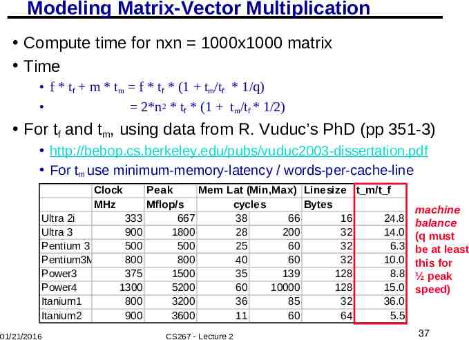
Modeling Matrix-Vector Multiplication Compute time for nxn 1000x1000 matrix Time f * tf m * tm f * tf * (1 tm/tf * 1/q) 2*n2 * tf * (1 tm/tf * 1/2) For tf and tm, using data from R. Vuduc’s PhD (pp 351-3) http://bebop.cs.berkeley.edu/pubs/vuduc2003-dissertation.pdf For tm use minimum-memory-latency / words-per-cache-line Clock MHz Ultra 2i Ultra 3 Pentium 3 Pentium3M Power3 Power4 Itanium1 Itanium2 01/21/2016 333 900 500 800 375 1300 800 900 Peak Mem Lat (Min,Max) Linesize t m/t f Mflop/s cycles Bytes 667 38 66 16 24.8 1800 28 200 32 14.0 500 25 60 32 6.3 800 40 60 32 10.0 1500 35 139 128 8.8 5200 60 10000 128 15.0 3200 36 85 32 36.0 3600 11 60 64 5.5 CS267 - Lecture 2 machine balance (q must be at least this for ½ peak speed) 37
Simplifying Assumptions What simplifying assumptions did we make in this analysis? Ignored parallelism in processor between memory and arithmetic within the processor Sometimes drop arithmetic term in this type of analysis Assumed fast memory was large enough to hold three vectors Reasonable if we are talking about any level of cache Not if we are talking about registers ( 32 words) Assumed the cost of a fast memory access is 0 Reasonable if we are talking about registers Not necessarily if we are talking about cache (1-2 cycles for L1) Memory latency is constant Could simplify even further by ignoring memory operations in X and Y vectors Mflop rate/element 2 / (2* tf tm) 01/21/2016 CS267 - Lecture 2 38
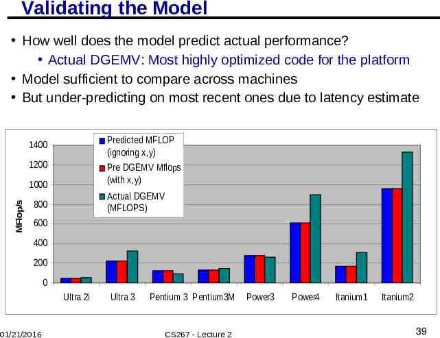
Validating the Model How well does the model predict actual performance? Actual DGEMV: Most highly optimized code for the platform Model sufficient to compare across machines But under-predicting on most recent ones due to latency estimate 1400 Predicted MFLOP (ignoring x,y) 1200 Pre DGEMV Mflops (with x,y) MFlop/s 1000 Actual DGEMV (MFLOPS) 800 600 400 200 0 Ultra 2i 01/21/2016 Ultra 3 Pentium 3 Pentium3M CS267 - Lecture 2 Power3 Power4 Itanium1 Itanium2 39
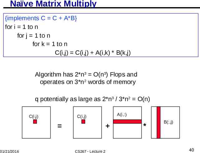
Naïve Matrix Multiply {implements C C A*B} for i 1 to n for j 1 to n for k 1 to n C(i,j) C(i,j) A(i,k) * B(k,j) Algorithm has 2*n3 O(n3) Flops and operates on 3*n2 words of memory q potentially as large as 2*n3 / 3*n2 O(n) C(i,j) 01/21/2016 A(i,:) C(i,j) CS267 - Lecture 2 * B(:,j) 40
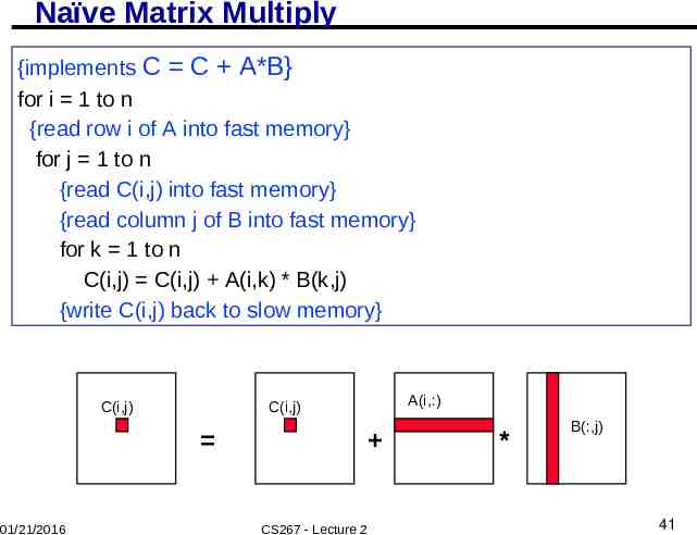
Naïve Matrix Multiply {implements C C A*B} for i 1 to n {read row i of A into fast memory} for j 1 to n {read C(i,j) into fast memory} {read column j of B into fast memory} for k 1 to n C(i,j) C(i,j) A(i,k) * B(k,j) {write C(i,j) back to slow memory} C(i,j) 01/21/2016 A(i,:) C(i,j) CS267 - Lecture 2 * B(:,j) 41
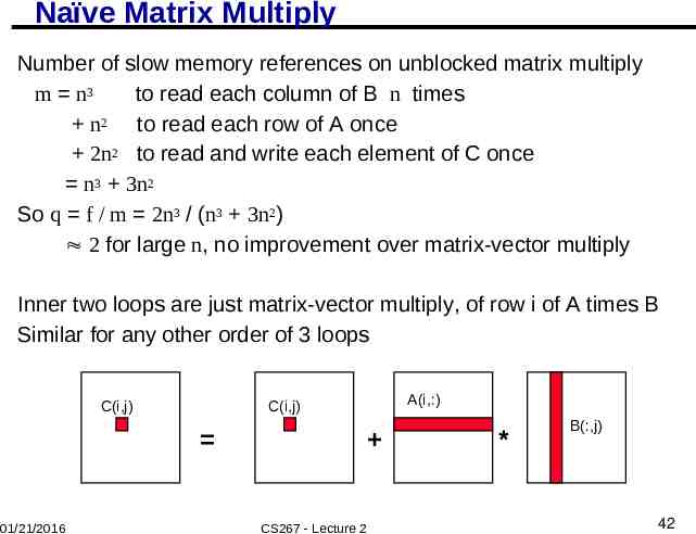
Naïve Matrix Multiply Number of slow memory references on unblocked matrix multiply m n3 to read each column of B n times n2 to read each row of A once 2n2 to read and write each element of C once n3 3n2 So q f / m 2n3 / (n3 3n2) 2 for large n, no improvement over matrix-vector multiply Inner two loops are just matrix-vector multiply, of row i of A times B Similar for any other order of 3 loops C(i,j) 01/21/2016 A(i,:) C(i,j) CS267 - Lecture 2 * B(:,j) 42
Matrix-multiply, optimized several ways Speed of n-by-n matrix multiply on Sun Ultra-1/170, peak 330 MFlops 01/21/2016 CS267 - Lecture 2 43
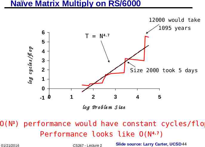
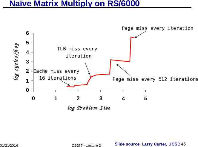
Naïve Matrix Multiply on RS/6000 12000 would take 1095 years 6 T N4.7 lo g c y c le s / fl o p 5 4 3 2 Size 2000 took 5 days 1 0 -1 0 1 2 3 4 5 lo g Pr o b le m S iz e O(N3) performance would have constant cycles/flop Performance looks like O(N4.7) 01/21/2016 CS267 - Lecture 2 Slide source: Larry Carter, UCSD 44
Naïve Matrix Multiply on RS/6000 Page miss every iteration lo g c y c le s / fl o p 6 5 TLB miss every iteration 4 3 2 Cache miss every 16 iterations 1 Page miss every 512 iterations 0 0 1 2 3 4 5 lo g Pr o b le m S iz e 01/21/2016 CS267 - Lecture 2 Slide source: Larry Carter, UCSD 45
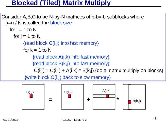
Blocked (Tiled) Matrix Multiply Consider A,B,C to be N-by-N matrices of b-by-b subblocks where b n / N is called the block size for i 1 to N for j 1 to N {read block C(i,j) into fast memory} for k 1 to N {read block A(i,k) into fast memory} {read block B(k,j) into fast memory} C(i,j) C(i,j) A(i,k) * B(k,j) {do a matrix multiply on blocks} {write block C(i,j) back to slow memory} C(i,j) 01/21/2016 A(i,k) C(i,j) CS267 - Lecture 2 * B(k,j) 46
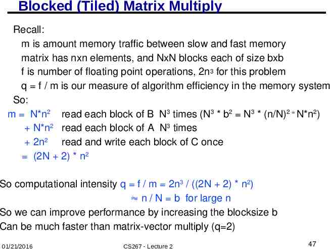
Blocked (Tiled) Matrix Multiply Recall: m is amount memory traffic between slow and fast memory matrix has nxn elements, and NxN blocks each of size bxb f is number of floating point operations, 2n3 for this problem q f / m is our measure of algorithm efficiency in the memory system So: m N*n2 read each block of B N3 times (N3 * b2 N3 * (n/N)2 N*n2) N*n2 read each block of A N3 times 2n2 read and write each block of C once (2N 2) * n2 So computational intensity q f / m 2n3 / ((2N 2) * n2) n / N b for large n So we can improve performance by increasing the blocksize b Can be much faster than matrix-vector multiply (q 2) 01/21/2016 CS267 - Lecture 2 47
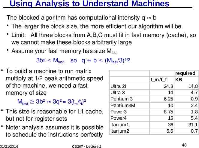
Using Analysis to Understand Machines The blocked algorithm has computational intensity q b The larger the block size, the more efficient our algorithm will be Limit: All three blocks from A,B,C must fit in fast memory (cache), so we cannot make these blocks arbitrarily large Assume your fast memory has size Mfast 3b2 Mfast, so q b (Mfast/3)1/2 To build a machine to run matrix multiply at 1/2 peak arithmetic speed of the machine, we need a fast memory of size Mfast 3b2 3q2 3(tm/tf)2 This size is reasonable for L1 cache, but not for register sets Note: analysis assumes it is possible to schedule the instructions perfectly 01/21/2016 CS267 - Lecture 2 Ultra 2i Ultra 3 Pentium 3 Pentium3M Power3 Power4 Itanium1 Itanium2 t m/t f 24.8 14 6.25 10 8.75 15 36 5.5 required KB 14.8 4.7 0.9 2.4 1.8 5.4 31.1 0.7 48
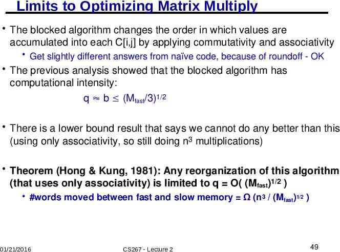
Limits to Optimizing Matrix Multiply The blocked algorithm changes the order in which values are accumulated into each C[i,j] by applying commutativity and associativity Get slightly different answers from naïve code, because of roundoff - OK The previous analysis showed that the blocked algorithm has computational intensity: q b (Mfast/3)1/2 There is a lower bound result that says we cannot do any better than this (using only associativity, so still doing n3 multiplications) Theorem (Hong & Kung, 1981): Any reorganization of this algorithm (that uses only associativity) is limited to q O( (Mfast)1/2 ) #words moved between fast and slow memory Ω (n3 / (Mfast)1/2 ) 01/21/2016 CS267 - Lecture 2 49
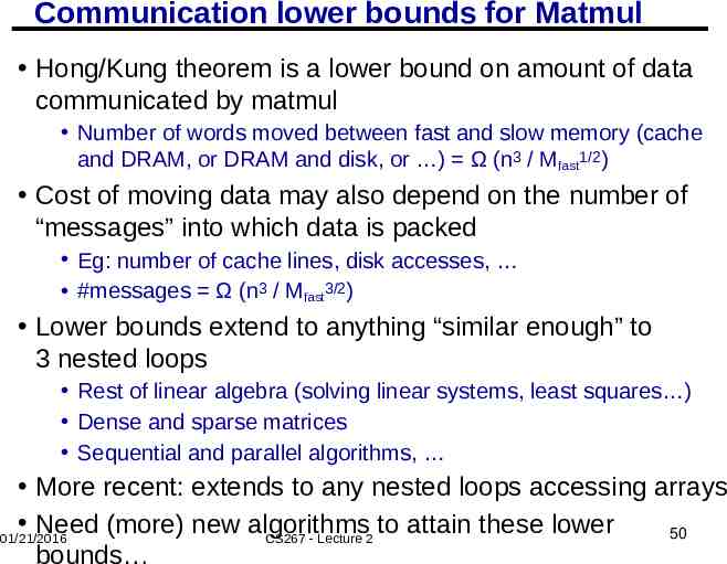
Communication lower bounds for Matmul Hong/Kung theorem is a lower bound on amount of data communicated by matmul Number of words moved between fast and slow memory (cache and DRAM, or DRAM and disk, or ) Ω (n3 / Mfast1/2) Cost of moving data may also depend on the number of “messages” into which data is packed Eg: number of cache lines, disk accesses, #messages Ω (n3 / Mfast3/2) Lower bounds extend to anything “similar enough” to 3 nested loops Rest of linear algebra (solving linear systems, least squares ) Dense and sparse matrices Sequential and parallel algorithms, More recent: extends to any nested loops accessing arrays Need (more) new algorithms to attain these lower 50 01/21/2016 CS267 - Lecture 2 bounds
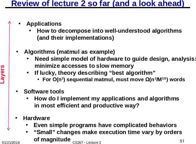
Review of lecture 2 so far (and a look ahead) Layers Applications How to decompose into well-understood algorithms (and their implementations) Algorithms (matmul as example) Need simple model of hardware to guide design, analysis: minimize accesses to slow memory If lucky, theory describing “best algorithm” For O(n3) sequential matmul, must move Ω(n3/M1/2) words Software tools How do I implement my applications and algorithms in most efficient and productive way? Hardware Even simple programs have complicated behaviors “Small” changes make execution time vary by orders of magnitude CS267 - Lecture 2 51 01/21/2016
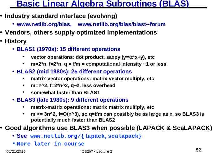
Basic Linear Algebra Subroutines (BLAS) Industry standard interface (evolving) www.netlib.org/blas, www.netlib.org/blas/blast--forum Vendors, others supply optimized implementations History BLAS1 (1970s): 15 different operations vector operations: dot product, saxpy (y *x y), etc m 2*n, f 2*n, q f/m computational intensity 1 or less BLAS2 (mid 1980s): 25 different operations matrix-vector operations: matrix vector multiply, etc m n 2, f 2*n 2, q 2, less overhead somewhat faster than BLAS1 BLAS3 (late 1980s): 9 different operations matrix-matrix operations: matrix matrix multiply, etc m 3n 2, f O(n 3), so q f/m can possibly be as large as n, so BLAS3 is potentially much faster than BLAS2 Good algorithms use BLAS3 when possible (LAPACK & ScaLAPACK) See www.netlib.org/{lapack,scalapack} More later in course 01/21/2016 CS267 - Lecture 2 52
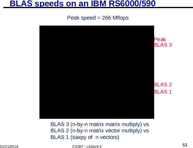
BLAS speeds on an IBM RS6000/590 Peak speed 266 Mflops Peak BLAS 3 BLAS 2 BLAS 1 BLAS 3 (n-by-n matrix matrix multiply) vs BLAS 2 (n-by-n matrix vector multiply) vs BLAS 1 (saxpy of n vectors) 01/21/2016 CS267 - Lecture 2 53
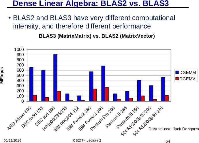
Dense Linear Algebra: BLAS2 vs. BLAS3 BLAS2 and BLAS3 have very different computational intensity, and therefore different performance MFlop/s BLAS3 (MatrixMatrix) vs. BLAS2 (MatrixVector) 1000 900 800 700 600 500 400 300 200 100 0 DGEMM DGEMV 50 00 00 60 00 66 33 12 00 00 70 35 5 5 6 5 1 2 2 1 1 2 2 2 5/ II623II6o804I r r r v 3 on 5 0 3 2 l e e P e 6 h ip ip /7 w w ev um ium C i 0 0 0 C m t o o At E n P P nt 00 00 00 tiu PP D EC e D e 0 2 9 n P M M D 1 1 Data source: Jack Dongarra P P M AM R R IB IB Pe H IB I I SG SG 01/21/2016 CS267 - Lecture 2 54
What if there are more than 2 levels of memory? Need to minimize communication between all levels Between L1 and L2 cache, cache and DRAM, DRAM and disk The tiled algorithm requires finding a good block size Machine dependent Need to “block” b x b matrix multiply in inner most loop 1 level of memory 3 nested loops (naïve algorithm) 2 levels of memory 6 nested loops 3 levels of memory 9 nested loops Cache Oblivious Algorithms offer an alternative Treat nxn matrix multiply as a set of smaller problems Eventually, these will fit in cache Will minimize # words moved between every level of memory hierarchy – at least asymptotically “Oblivious” to number and sizes of levels 01/21/2016 CS267 - Lecture 2 55
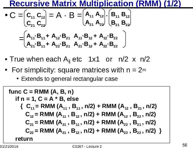
Recursive Matrix Multiplication (RMM) (1/2) C C11 C12 A · B A11 A12 · B11 B12 C21 C22 A21 A22 B21 B22 A11·B11 A12·B21 A11·B12 A12·B22 A21·B11 A22·B21 A21·B12 A22·B22 True when each Aij etc 1x1 or n/2 x n/2 For simplicity: square matrices with n 2m Extends to general rectangular case func C RMM (A, B, n) if n 1, C A * B, else { C11 RMM (A11 , B11 , n/2) RMM (A12 , B21 , n/2) C12 RMM (A11 , B12 , n/2) RMM (A12 , B22 , n/2) C21 RMM (A21 , B11 , n/2) RMM (A22 , B21 , n/2) C22 RMM (A21 , B12 , n/2) RMM (A22 , B22 , n/2) } return 01/21/2016 CS267 - Lecture 2 56
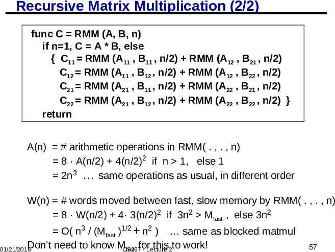
Recursive Matrix Multiplication (2/2) func C RMM (A, B, n) if n 1, C A * B, else { C11 RMM (A11 , B11 , n/2) RMM (A12 , B21 , n/2) C12 RMM (A11 , B12 , n/2) RMM (A12 , B22 , n/2) C21 RMM (A21 , B11 , n/2) RMM (A22 , B21 , n/2) C22 RMM (A21 , B12 , n/2) RMM (A22 , B22 , n/2) } return A(n) # arithmetic operations in RMM( . , . , n) 8 · A(n/2) 4(n/2)2 if n 1, else 1 2n3 same operations as usual, in different order W(n) # words moved between fast, slow memory by RMM( . , . , n) 8 · W(n/2) 4· 3(n/2)2 if 3n2 Mfast , else 3n2 O( n3 / (Mfast )1/2 n2 ) same as blocked matmul Don’t need to know MCS267 this2to work! fast for 01/21/2016 - Lecture 57
Experience with Cache-Oblivious Algorithms In practice, need to cut off recursion well before 1x1 blocks Call “micro-kernel” on small blocks Implementing high-performance Cache-Oblivious code not easy Careful attention to micro-kernel is needed Using fully recursive approach with highly optimized recursive micro-kernel, Pingali et al report that they never got more than 2/3 of peak. (unpublished, presented at LACSI’06) Issues with Cache Oblivious (recursive) approach Recursive Micro-Kernels yield less performance than iterative ones using same scheduling techniques Pre-fetching is needed to compete with best code: not well-understood in the context of Cache-Oblivious codes More recent work on CARMA (UCB) uses recursion for parallelism, but aware of available memory, very fast (later) Up to 6.6x faster than Intel MKL for some matrix shapes, 17% for square 01/21/2016 CS267 - Lecture 2
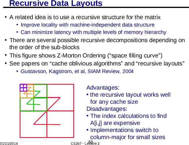
Recursive Data Layouts A related idea is to use a recursive structure for the matrix Improve locality with machine-independent data structure Can minimize latency with multiple levels of memory hierarchy There are several possible recursive decompositions depending on the order of the sub-blocks This figure shows Z-Morton Ordering (“space filling curve”) See papers on “cache oblivious algorithms” and “recursive layouts” Gustavson, Kagstrom, et al, SIAM Review, 2004 Advantages: the recursive layout works well for any cache size Disadvantages: The index calculations to find A[i,j] are expensive Implementations switch to column-major for small sizes 01/21/2016 60 2 CS267 - Lecture
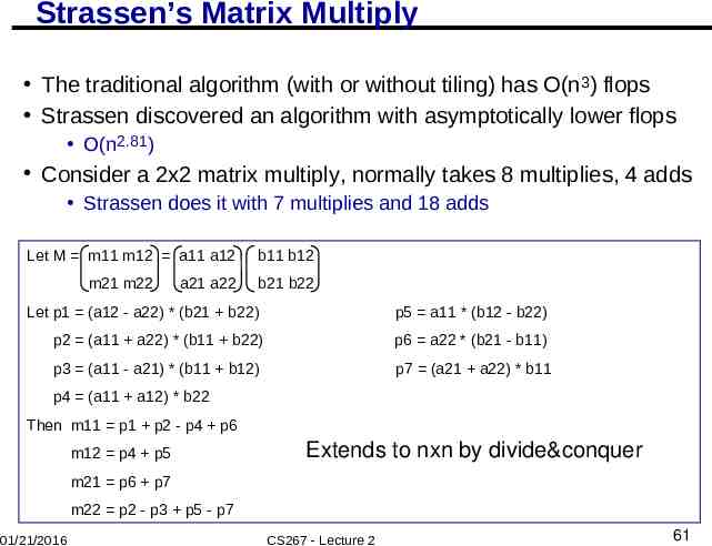
Strassen’s Matrix Multiply The traditional algorithm (with or without tiling) has O(n3) flops Strassen discovered an algorithm with asymptotically lower flops O(n2.81) Consider a 2x2 matrix multiply, normally takes 8 multiplies, 4 adds Strassen does it with 7 multiplies and 18 adds Let M m11 m12 a11 a12 b11 b12 m21 m22 a21 a22 b21 b22 Let p1 (a12 - a22) * (b21 b22) p5 a11 * (b12 - b22) p2 (a11 a22) * (b11 b22) p6 a22 * (b21 - b11) p3 (a11 - a21) * (b11 b12) p7 (a21 a22) * b11 p4 (a11 a12) * b22 Then m11 p1 p2 - p4 p6 m12 p4 p5 Extends to nxn by divide&conquer m21 p6 p7 m22 p2 - p3 p5 - p7 01/21/2016 CS267 - Lecture 2 61
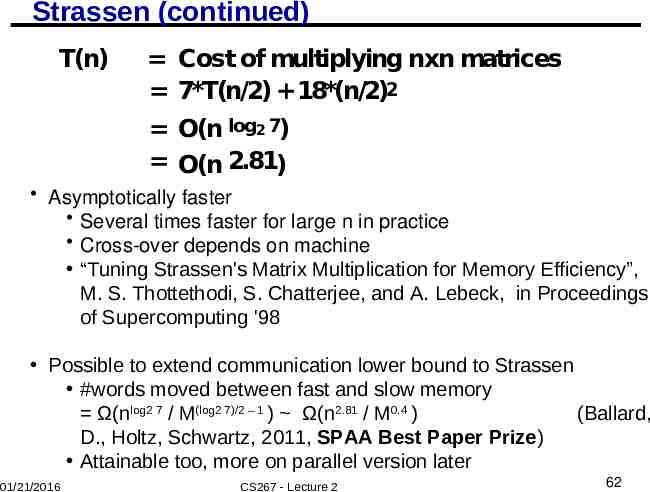
Strassen (continued) T(n) Cost of multiplying nxn matrices 7*T(n/2) 18*(n/2)2 O(n log2 7) O(n 2.81) Asymptotically faster Several times faster for large n in practice Cross-over depends on machine “Tuning Strassen's Matrix Multiplication for Memory Efficiency”, M. S. Thottethodi, S. Chatterjee, and A. Lebeck, in Proceedings of Supercomputing '98 Possible to extend communication lower bound to Strassen #words moved between fast and slow memory Ω(nlog2 7 / M(log2 7)/2 – 1 ) Ω(n2.81 / M0.4 ) (Ballard, D., Holtz, Schwartz, 2011, SPAA Best Paper Prize) Attainable too, more on parallel version later 01/21/2016 CS267 - Lecture 2 62
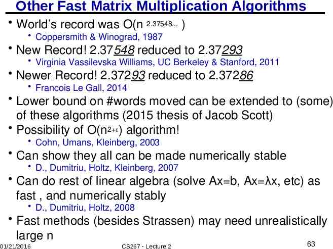
Other Fast Matrix Multiplication Algorithms World’s record was O(n 2.37548. ) Coppersmith & Winograd, 1987 New Record! 2.37548 reduced to 2.37293 Virginia Vassilevska Williams, UC Berkeley & Stanford, 2011 Newer Record! 2.37293 reduced to 2.37286 Francois Le Gall, 2014 Lower bound on #words moved can be extended to (some) of these algorithms (2015 thesis of Jacob Scott) Possibility of O(n2 ) algorithm! Cohn, Umans, Kleinberg, 2003 Can show they all can be made numerically stable D., Dumitriu, Holtz, Kleinberg, 2007 Can do rest of linear algebra (solve Ax b, Ax λx, etc) as fast , and numerically stably D., Dumitriu, Holtz, 2008 Fast methods (besides Strassen) may need unrealistically large n 01/21/2016 CS267 - Lecture 2 63
Tuning Code in Practice Tuning code can be tedious Lots of code variations to try besides blocking Machine hardware performance hard to predict Compiler behavior hard to predict Response: “Autotuning” Let computer generate large set of possible code variations, and search them for the fastest ones Used with CS267 homework assignment in mid 1990s PHiPAC, leading to ATLAS, incorporated in Matlab We still use the same assignment We (and others) are extending autotuning to other dwarfs / motifs, eg FFT Sometimes all done “off-line”, sometimes at run-time Still need to understand how to do it by hand Not every code will have an autotuner Need to know if you want to build autotuners 01/21/2016 CS267 - Lecture 2 64
Search Over Block Sizes Performance models are useful for high level algorithms Helps in developing a blocked algorithm Models have not proven very useful for block size selection too complicated to be useful – See work by Sid Chatterjee for detailed model too simple to be accurate – Multiple multidimensional arrays, virtual memory, etc. Speed depends on matrix dimensions, details of code, compiler, processor 01/21/2016 CS267 - Lecture 2 65
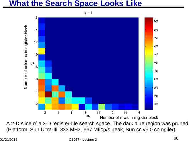
Number of columns in register block What the Search Space Looks Like Number of rows in register block A 2-D slice of a 3-D register-tile search space. The dark blue region was pruned. (Platform: Sun Ultra-IIi, 333 MHz, 667 Mflop/s peak, Sun cc v5.0 compiler) 01/21/2016 CS267 - Lecture 2 66
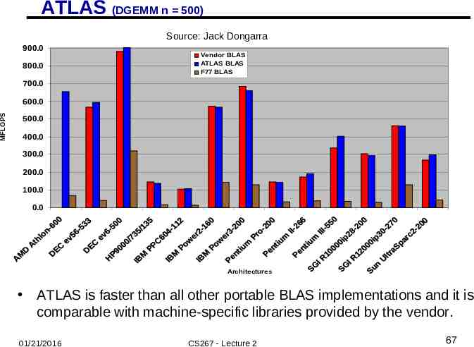
ATLAS (DGEMM n 500) Source: Jack Dongarra 900.0 800.0 Vendor BLAS ATLAS BLAS F77 BLAS 700.0 MFLOPS 600.0 500.0 400.0 300.0 200.0 100.0 0.0 Architectures ATLAS is faster than all other portable BLAS implementations and it is comparable with machine-specific libraries provided by the vendor. 01/21/2016 CS267 - Lecture 2 67
Optimizing in Practice Tiling for registers loop unrolling, use of named “register” variables Tiling for multiple levels of cache and TLB Exploiting fine-grained parallelism in processor superscalar; pipelining Complicated compiler interactions (flags) Hard to do by hand (but you’ll try) Automatic optimization an active research area ASPIRE: aspire.eecs.berkeley.edu BeBOP: bebop.cs.berkeley.edu Weekly group meeting Mondays 1pm PHiPAC: www.icsi.berkeley.edu/ bilmes/phipac in particular tr-98-035.ps.gz ATLAS: www.netlib.org/atlas 01/21/2016 CS267 - Lecture 2 68
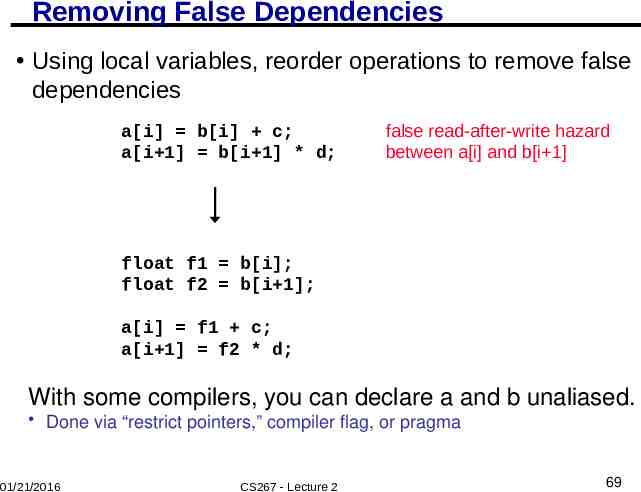
Removing False Dependencies Using local variables, reorder operations to remove false dependencies a[i] b[i] c; a[i 1] b[i 1] * d; false read-after-write hazard between a[i] and b[i 1] float f1 b[i]; float f2 b[i 1]; a[i] f1 c; a[i 1] f2 * d; With some compilers, you can declare a and b unaliased. Done via “restrict pointers,” compiler flag, or pragma 01/21/2016 CS267 - Lecture 2 69
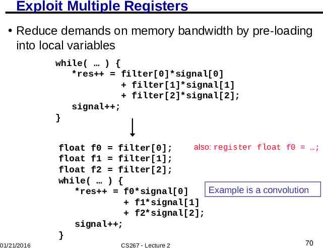
Exploit Multiple Registers Reduce demands on memory bandwidth by pre-loading into local variables while( ) { *res filter[0]*signal[0] filter[1]*signal[1] filter[2]*signal[2]; signal ; } also: register float f0 ; float f0 filter[0]; float f1 filter[1]; float f2 filter[2]; while( ) { Example is a convolution *res f0*signal[0] f1*signal[1] f2*signal[2]; signal ; } 01/21/2016 CS267 - Lecture 2 70
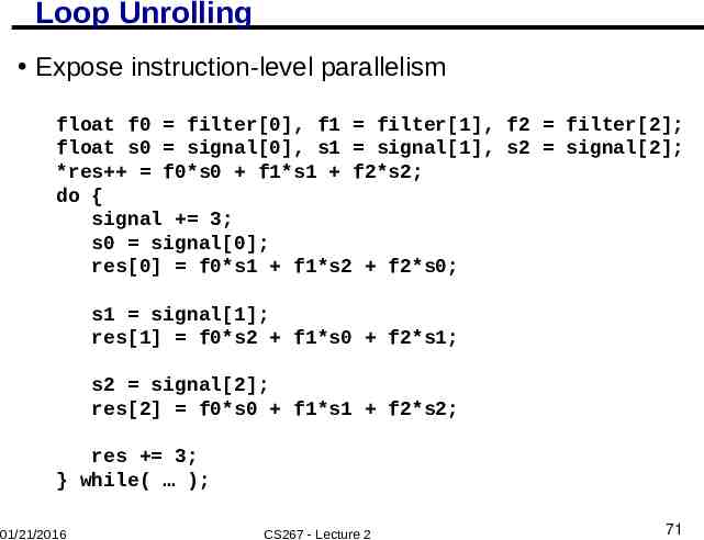
Loop Unrolling Expose instruction-level parallelism float f0 filter[0], f1 filter[1], f2 filter[2]; float s0 signal[0], s1 signal[1], s2 signal[2]; *res f0*s0 f1*s1 f2*s2; do { signal 3; s0 signal[0]; res[0] f0*s1 f1*s2 f2*s0; s1 signal[1]; res[1] f0*s2 f1*s0 f2*s1; s2 signal[2]; res[2] f0*s0 f1*s1 f2*s2; res 3; } while( ); 01/21/2016 CS267 - Lecture 2 71
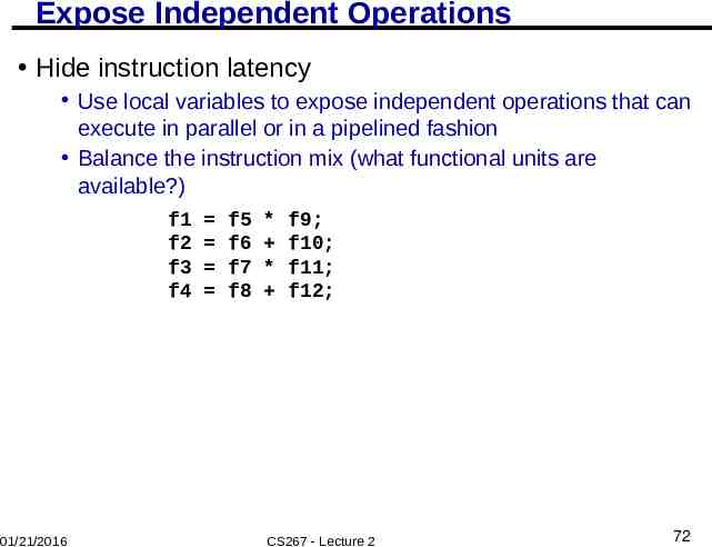
Expose Independent Operations Hide instruction latency Use local variables to expose independent operations that can execute in parallel or in a pipelined fashion Balance the instruction mix (what functional units are available?) f1 f2 f3 f4 01/21/2016 f5 f6 f7 f8 * * f9; f10; f11; f12; CS267 - Lecture 2 72
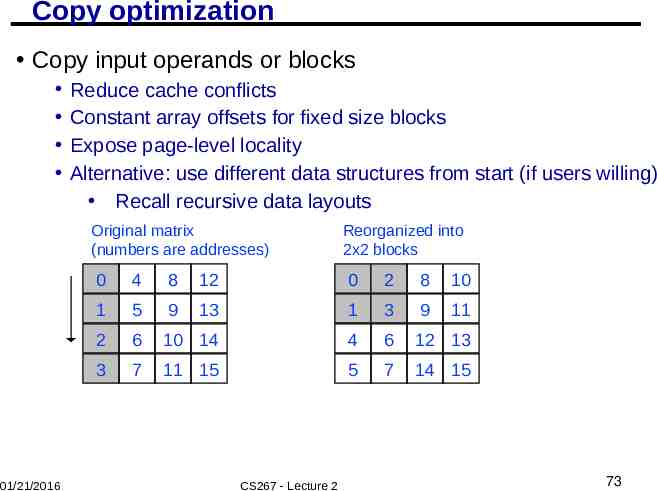
Copy optimization Copy input operands or blocks Reduce cache conflicts Constant array offsets for fixed size blocks Expose page-level locality Alternative: use different data structures from start (if users willing) Recall recursive data layouts Original matrix (numbers are addresses) 01/21/2016 Reorganized into 2x2 blocks 0 4 8 12 0 2 8 10 1 5 9 13 1 3 9 11 2 6 10 14 4 6 12 13 3 7 11 15 5 7 14 15 CS267 - Lecture 2 73
Locality in Other Algorithms The performance of any algorithm is limited by q q “computational intensity” #arithmetic ops / #words moved In matrix multiply, we increase q by changing computation order increased temporal locality For other algorithms and data structures, even handtransformations are still an open problem Lots of open problems, class projects 01/21/2016 CS267 - Lecture 2 74
Summary of Lecture 2 Details of machine are important for performance Processor and memory system (not just parallelism) Before you parallelize, make sure you’re getting good serial performance What to expect? Use understanding of hardware limits There is parallelism hidden within processors Pipelining, SIMD, etc Machines have memory hierarchies 100s of cycles to read from DRAM (main memory) Caches are fast (small) memory that optimize average case Locality is at least as important as computation Temporal: re-use of data recently used Spatial: using data nearby to recently used data Can rearrange code/data to improve locality Goal: minimize communication data movement 01/21/2016 CS267 - Lecture 2 75
Class Logistics Homework 0 posted on web site Find and describe interesting application of parallelism Due Friday Jan 29 Could even be your intended class project Please fill in on-line class survey by midnight Jan 28 We need this to assign teams for Homework 1 Teams will be announced Friday morning Jan 29, when HW 1 is posted Please fill out on-line request for Stampede account Needed for GPU part of assignment 2 Also has Intel Xeon-Phi 01/21/2016 CS267 - Lecture 2 76
Some reading for today (see website) Sourcebook Chapter 3, (note that chapters 2 and 3 cover the material of lecture 2 and lecture 3, but not in the same order). "Performance Optimization of Numerically Intensive Codes", by Stefan Goedecker and Adolfy Hoisie, SIAM 2001. Web pages for reference: BeBOP Homepage ATLAS Homepage BLAS (Basic Linear Algebra Subroutines), Reference for (unoptimized) implementations of the BLAS, with documentation. LAPACK (Linear Algebra PACKage), a standard linear algebra library optimized to use the BLAS effectively on uniprocessors and shared memory machines (software, documentation and reports) ScaLAPACK (Scalable LAPACK), a parallel version of LAPACK for distributed memory machines (software, documentation and reports) Tuning Strassen's Matrix Multiplication for Memory Efficiency Mithuna S. Thottethodi, Siddhartha Chatterjee, and Alvin R. Lebeck in Proceedings of Supercomputing '98, November 1998 postscript Recursive Array Layouts and Fast Parallel Matrix Multiplication” by Chatterjee et al. IEEE TPDS November 2002. Many related papers at bebop.cs.berkeley.edu 01/21/2016 CS267 - Lecture 2 77
Extra Slides 01/21/2016 CS267 - Lecture 2 78