CONTROL CHART FOR QUALITY CONTROL X-R CHART X-R chart is a pair

19 Slides802.00 KB
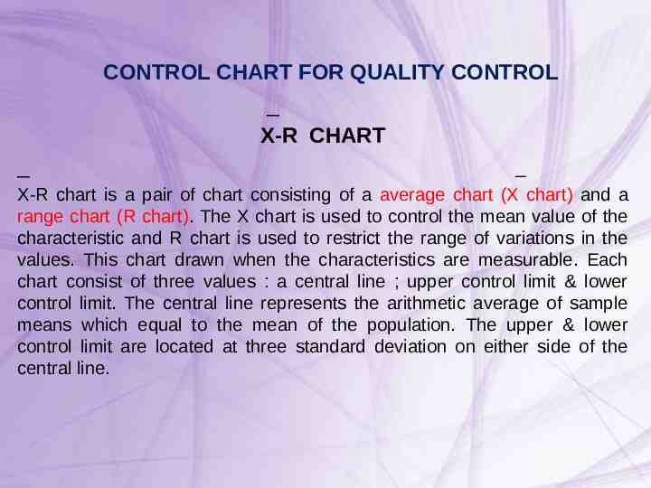
CONTROL CHART FOR QUALITY CONTROL X-R CHART X-R chart is a pair of chart consisting of a average chart (X chart) and a range chart (R chart). The X chart is used to control the mean value of the characteristic and R chart is used to restrict the range of variations in the values. This chart drawn when the characteristics are measurable. Each chart consist of three values : a central line ; upper control limit & lower control limit. The central line represents the arithmetic average of sample means which equal to the mean of the population. The upper & lower control limit are located at three standard deviation on either side of the central line.
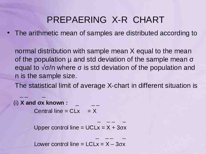
PREPAERING X-R CHART The arithmetic mean of samples are distributed according to normal distribution with sample mean X equal to the mean of the population µ and std deviation of the sample mean σ equal to σ/n where σ is std deviation of the population and n is the sample size. The statistical limit of average X-chart in different situation is (i) X and σx known : Central line CLx X Upper control line UCLx X 3σx Lower control line LCLx X – 3σx
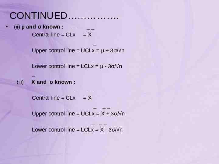
CONTINUED . (ii) µ and σ known : Central line CLx (iii) X Upper control line UCLx µ 3σ/ n Lower control line LCLx µ - 3σ/ n X and σ known : Central line CLx X Upper control line UCLx X 3σ/ n Lower control line LCLx X - 3σ/ n
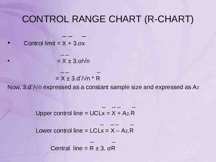
CONTROL RANGE CHART (R-CHART) Control limit X 3.σx X 3.σ/ n X 3.d / n * R Now, 3.d / n expressed as a constant sample size and expressed as A2 Upper control line UCLx X A2.R Lower control line LCLx X – A2.R Central line R 3. σR
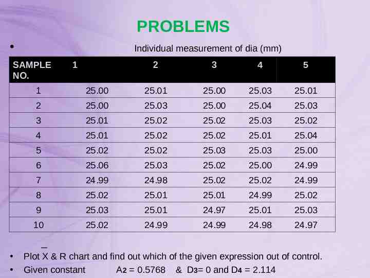
PROBLEMS Individual measurement of dia (mm) SAMPLE NO. 1 2 3 4 5 1 25.00 25.01 25.00 25.03 25.01 2 25.00 25.03 25.00 25.04 25.03 3 25.01 25.02 25.02 25.03 25.02 4 25.01 25.02 25.02 25.01 25.04 5 25.02 25.02 25.03 25.03 25.00 6 25.06 25.03 25.02 25.00 24.99 7 24.99 24.98 25.02 25.02 24.99 8 25.02 25.01 25.01 24.99 25.02 9 25.03 25.01 24.97 25.01 25.03 10 25.02 24.99 24.99 24.98 24.97 Plot X & R chart and find out which of the given expression out of control. Given constant A2 0.5768 & D3 0 and D4 2.114
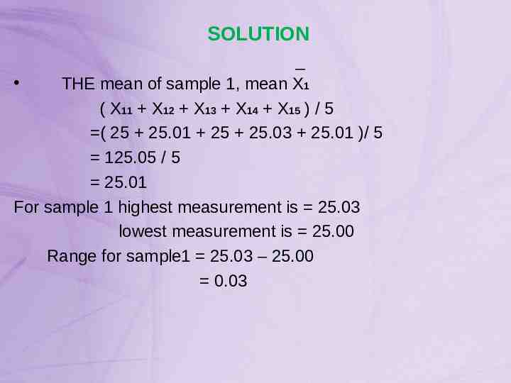
SOLUTION THE mean of sample 1, mean X1 ( X11 X12 X13 X14 X15 ) / 5 ( 25 25.01 25 25.03 25.01 )/ 5 125.05 / 5 25.01 For sample 1 highest measurement is 25.03 lowest measurement is 25.00 Range for sample1 25.03 – 25.00 0.03
Arithmetic mean & range of sample table SAMPLE NUMBER ARITHMETIC MEAN RANGE 1 25.01 0.03 2 25.02 0.04 3 25.02 0.02 4 25.02 0.03 5 25.02 0.03 6 25.02 0.07 7 25.00 0.04 8 25.01 0.03 9 25.01 0.06 10 24.98 0.05
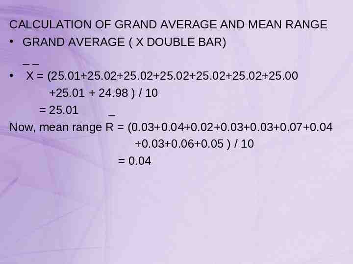
CALCULATION OF GRAND AVERAGE AND MEAN RANGE GRAND AVERAGE ( X DOUBLE BAR) X (25.01 25.02 25.02 25.02 25.02 25.02 25.00 25.01 24.98 ) / 10 25.01 Now, mean range R (0.03 0.04 0.02 0.03 0.03 0.07 0.04 0.03 0.06 0.05 ) / 10 0.04
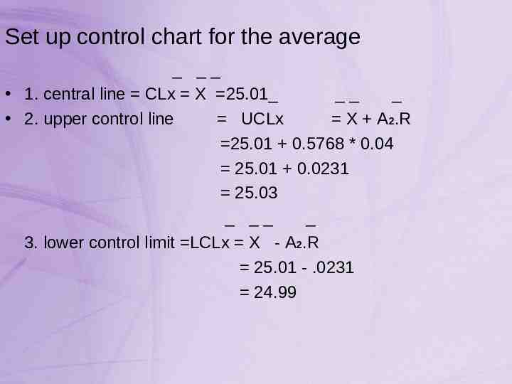
Set up control chart for the average 1. central line CLx X 25.01 2. upper control line UCLx X A2.R 25.01 0.5768 * 0.04 25.01 0.0231 25.03 3. lower control limit LCLx X - A2.R 25.01 - .0231 24.99
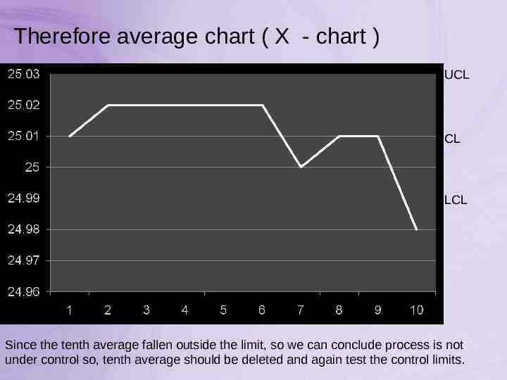
Therefore average chart ( X - chart ) UCL CL LCL Since the tenth average fallen outside the limit, so we can conclude process is not under control so, tenth average should be deleted and again test the control limits.
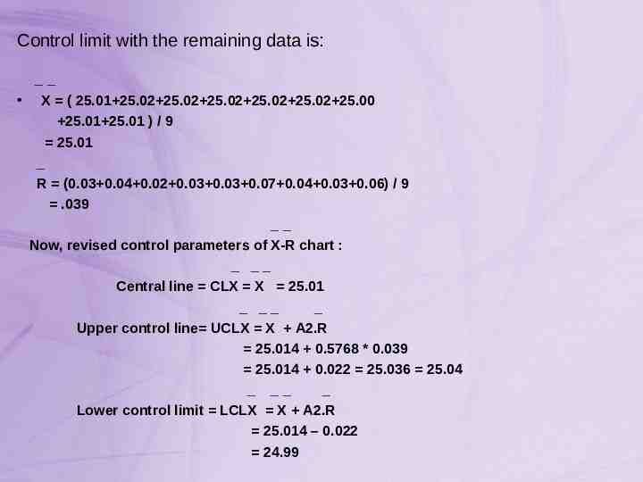
Control limit with the remaining data is: X ( 25.01 25.02 25.02 25.02 25.02 25.02 25.00 25.01 25.01 ) / 9 25.01 R (0.03 0.04 0.02 0.03 0.03 0.07 0.04 0.03 0.06) / 9 .039 Now, revised control parameters of X-R chart : Central line CLX X 25.01 Upper control line UCLX X A2.R 25.014 0.5768 * 0.039 25.014 0.022 25.036 25.04 Lower control limit LCLX X A2.R 25.014 – 0.022 24.99
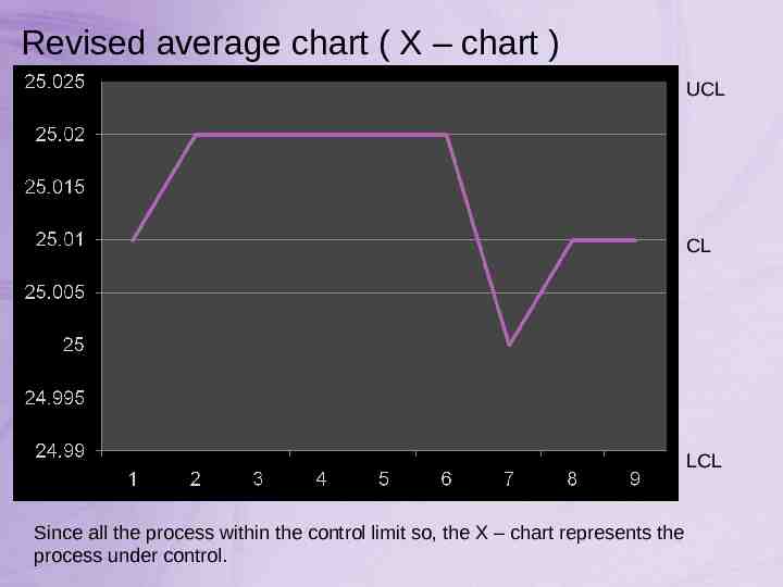
Revised average chart ( X – chart ) UCL CL LCL Since all the process within the control limit so, the X – chart represents the process under control.
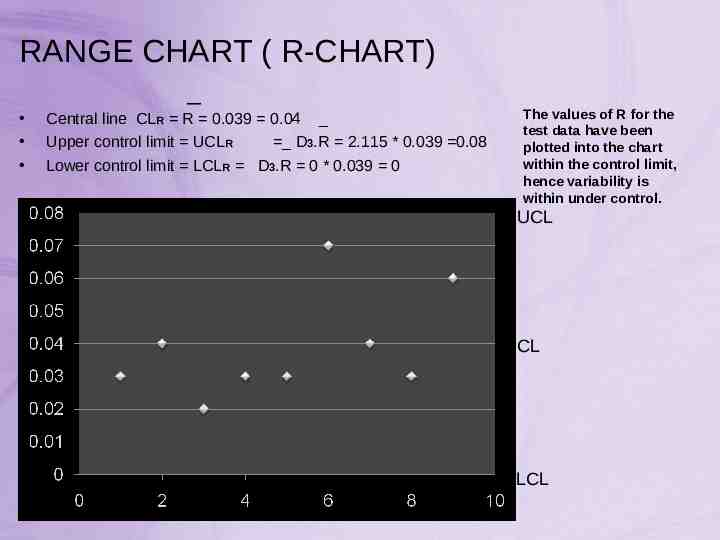
RANGE CHART ( R-CHART) Central line CLR R 0.039 0.04 Upper control limit UCLR D3.R 2.115 * 0.039 0.08 Lower control limit LCLR D3.R 0 * 0.039 0 The values of R for the test data have been plotted into the chart within the control limit, hence variability is within under control. UCL CL LCL
CONTROL CHART FOR ATTRIBUTE(p-CHART) Another form of inspection is where the items comprising the sample are classified into two types : ‘acceptable’ & ‘nonacceptable’ such as inspection is known as “inspection by attributes”. Inspection by attribute covers those situations where either : (i) quantitative measurement are not possible as with the inspection of damages, scratches, paint runs, matching of colour against std. shade etc. (ii) quantitative measurement consumes too much time. The control chart which do this kinds of inspection is known as control chart for fraction defectives ( p-Chart)
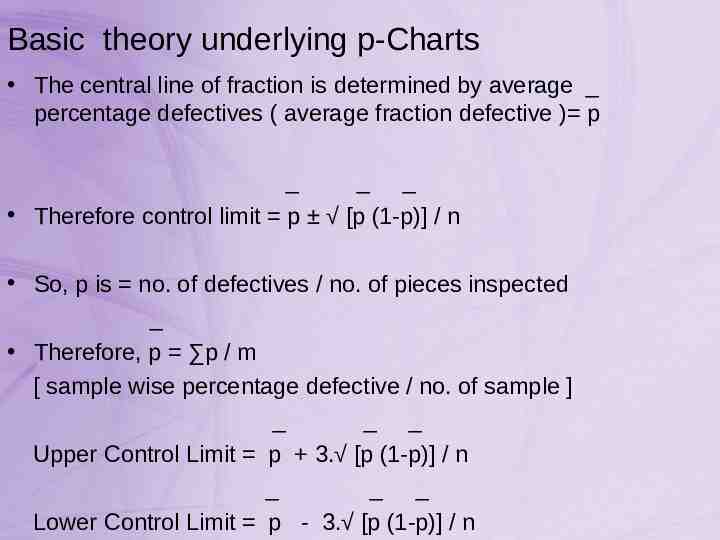
Basic theory underlying p-Charts The central line of fraction is determined by average percentage defectives ( average fraction defective ) p Therefore control limit p [p (1-p)] / n So, p is no. of defectives / no. of pieces inspected Therefore, p p / m [ sample wise percentage defective / no. of sample ] Upper Control Limit p 3. [p (1-p)] / n Lower Control Limit p - 3. [p (1-p)] / n
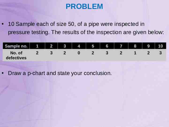
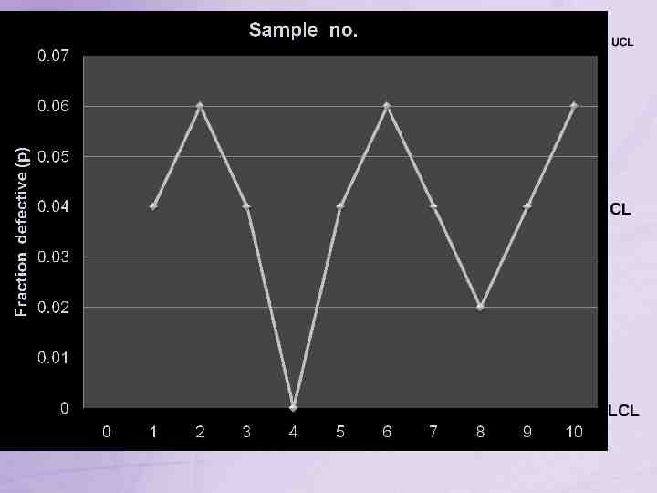
PROBLEM 10 Sample each of size 50, of a pipe were inspected in pressure testing. The results of the inspection are given below: Sample no. 1 2 3 4 5 6 7 8 9 10 No. of defectives 2 3 2 0 2 3 2 1 2 3 Draw a p-chart and state your conclusion.
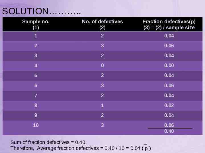
SOLUTION . Sample no. (1) No. of defectives (2) Fraction defectives(p) (3) (2) / sample size 1 2 0.04 2 3 0.06 3 2 0.04 4 0 0.00 5 2 0.04 6 3 0.06 7 2 0.04 8 1 0.02 9 2 0.04 10 3 0.06 0.40 Sum of fraction defectives 0.40 Therefore, Average fraction defectives 0.40 / 10 0.04 ( p )
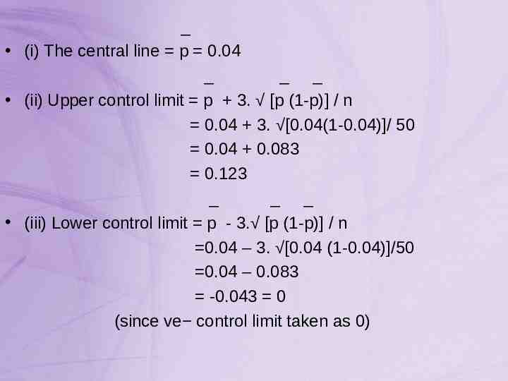
(i) The central line p 0.04 (ii) Upper control limit p 3. [p (1-p)] / n 0.04 3. [0.04(1-0.04)]/ 50 0.04 0.083 0.123 (iii) Lower control limit p - 3. [p (1-p)] / n 0.04 – 3. [0.04 (1-0.04)]/50 0.04 – 0.083 -0.043 0 (since ve control limit taken as 0)
UCL CL LCL