Application of spatial autocorrelation analysis in determining
25 Slides8.26 MB
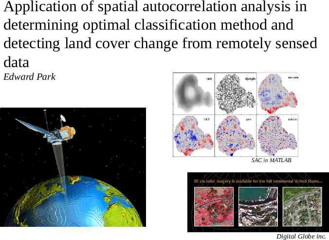
Application of spatial autocorrelation analysis in determining optimal classification method and detecting land cover change from remotely sensed data Edward Park SAC in MATLAB Digital Globe inc.
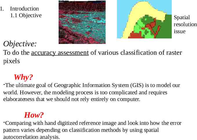
1. Introduction 1.1 Objective Spatial resolution issue Objective: To do the accuracy assessment of various classification of raster pixels Why? -The ultimate goal of Geographic Information System (GIS) is to model our world. However, the modeling process is too complicated and requires elaborateness that we should not rely entirely on computer. How? -Comparing with hand digitized reference image and look into how the error pattern varies depending on classification methods by using spatial autocorrelation analysis.
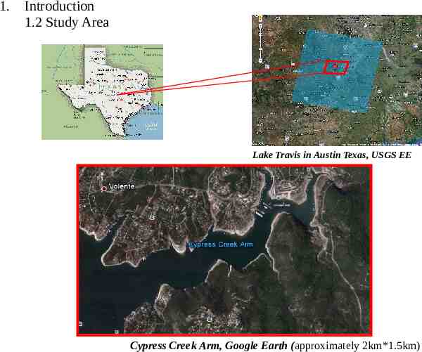
1. Introduction 1.2 Study Area Lake Travis in Austin Texas, USGS EE Cypress Creek Arm, Google Earth (approximately 2km*1.5km)
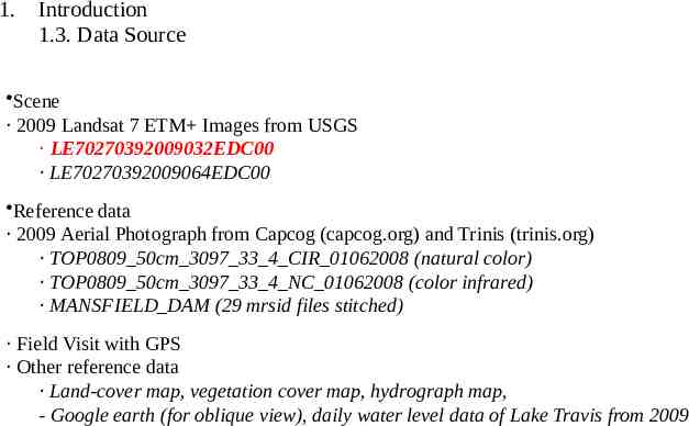
1. Introduction 1.3. Data Source Scene · 2009 Landsat 7 ETM Images from USGS · LE70270392009032EDC00 · LE70270392009064EDC00 Reference data · 2009 Aerial Photograph from Capcog (capcog.org) and Trinis (trinis.org) · TOP0809 50cm 3097 33 4 CIR 01062008 (natural color) · TOP0809 50cm 3097 33 4 NC 01062008 (color infrared) · MANSFIELD DAM (29 mrsid files stitched) · Field Visit with GPS · Other reference data · Land-cover map, vegetation cover map, hydrograph map, - Google earth (for oblique view), daily water level data of Lake Travis from 2009
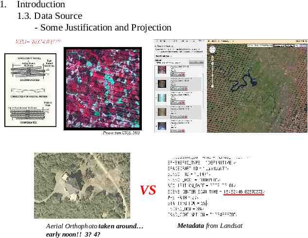
1. Introduction 1.3. Data Source - Some Justification and Projection VS Aerial Orthophoto taken around early noon!! 3? 4? Metadata from Landsat
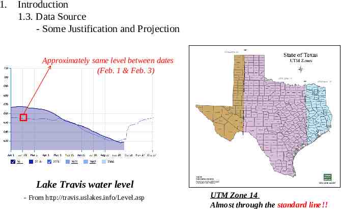
1. Introduction 1.3. Data Source - Some Justification and Projection Approximately same level between dates (Feb. 1 & Feb. 3) Lake Travis water level - From http://travis.uslakes.info/Level.asp UTM Zone 14 Almost through the standard line!!
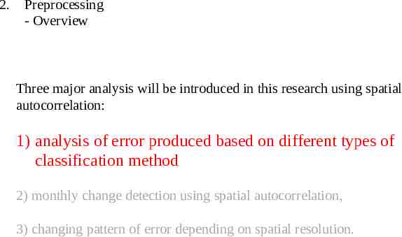
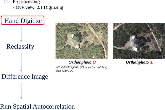
2. Preprocessing - Overview Three major analysis will be introduced in this research using spatial autocorrelation: 1) analysis of error produced based on different types of classification method 2) monthly change detection using spatial autocorrelation, 3) changing pattern of error depending on spatial resolution.
2. Preprocessing - Overview, 2.1 Digitizing Hand Digitize Reclassify Orthohphoto O MANSFIELD DAM (29 mrsid files stitched) from CAPCOG Difference Image Run Spatial Autocorrelation Orthohphoto X
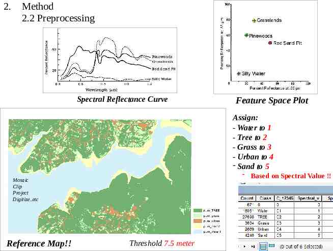
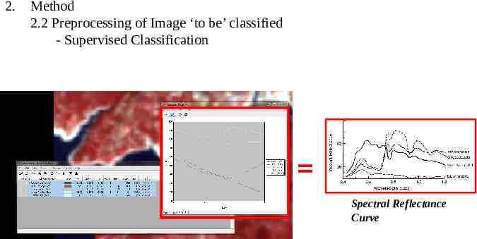
2. Method 2.2 Preprocessing Spectral Reflectance Curve Feature Space Plot Assign: - Water to 1 - Tree to 2 - Grass to 3 - Urban to 4 - Sand to 5 - Based on Spectral Value !! Mosaic Clip Project Digitize.etc Reference Map!! Threshold 7.5 meter
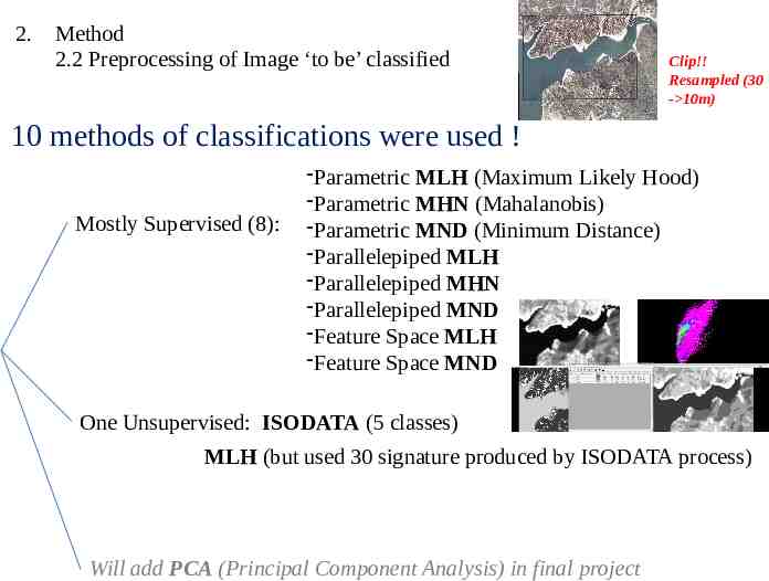
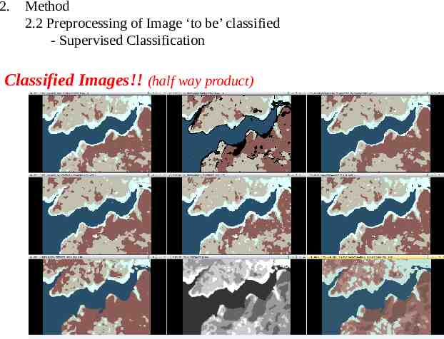
2. Method 2.2 Preprocessing of Image ‘to be’ classified Clip!! Resampled (30 - 10m) 10 methods of classifications were used ! Mostly Supervised (8): -Parametric MLH (Maximum Likely Hood) -Parametric MHN (Mahalanobis) -Parametric MND (Minimum Distance) -Parallelepiped MLH -Parallelepiped MHN -Parallelepiped MND -Feature Space MLH -Feature Space MND One Unsupervised: ISODATA (5 classes) MLH (but used 30 signature produced by ISODATA process) Will add PCA (Principal Component Analysis) in final project
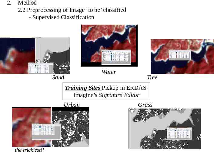
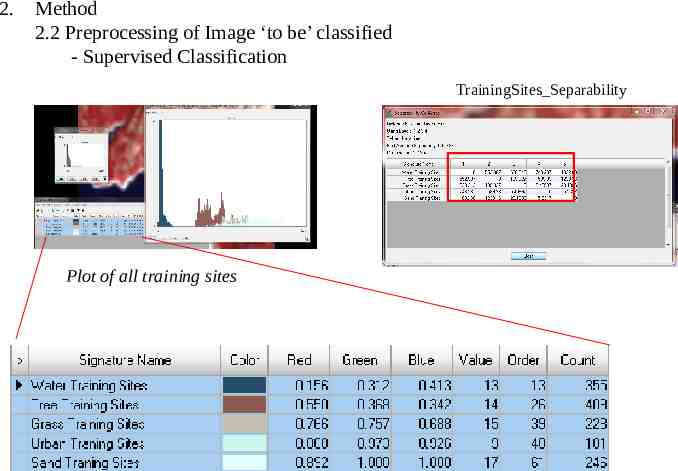
2. Method 2.2 Preprocessing of Image ‘to be’ classified - Supervised Classification Water Sand Tree Training Sites Pickup in ERDAS Imagine’s Signature Editor Urban the trickiest!! Grass
2. Method 2.2 Preprocessing of Image ‘to be’ classified - Supervised Classification TrainingSites Separability Plot of all training sites
2. Method 2.2 Preprocessing of Image ‘to be’ classified - Supervised Classification Spectral Reflectance Curve
2. Method 2.2 Preprocessing of Image ‘to be’ classified - Supervised Classification Classified Images!! (half way product)
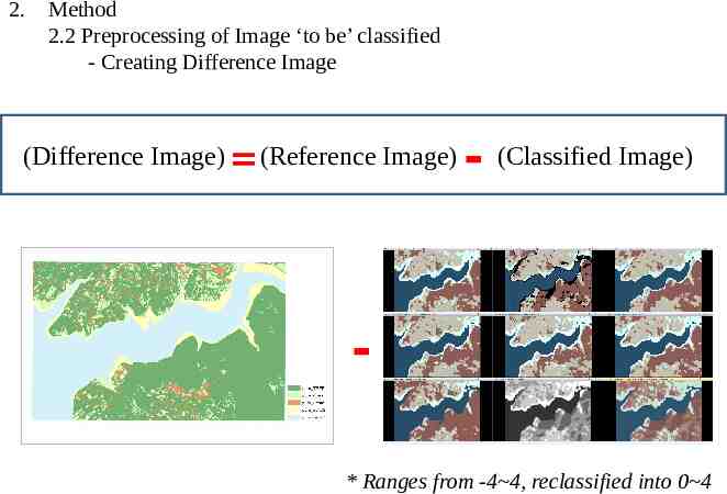
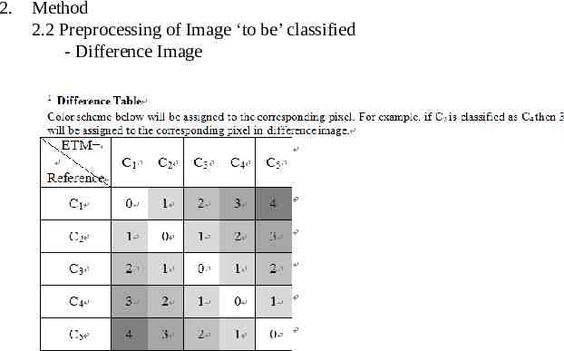
2. Method 2.2 Preprocessing of Image ‘to be’ classified - Creating Difference Image (Difference Image) (Reference Image) - (Classified Image) * Ranges from -4 4, reclassified into 0 4
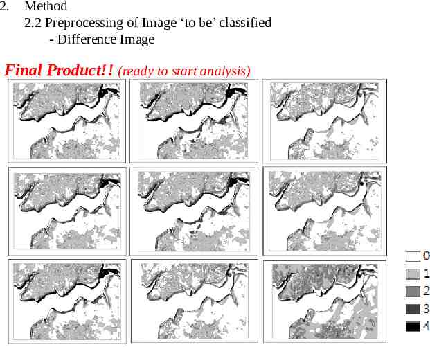
2. Method 2.2 Preprocessing of Image ‘to be’ classified - Difference Image
2. Method 2.2 Preprocessing of Image ‘to be’ classified - Difference Image Final Product!! (ready to start analysis) One Unsupervised: One Unsupervised:
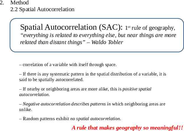
2. Method 2.2 Spatial Autocorrelation Spatial Autocorrelation (SAC): 1st rule of geography, “everything is related to everything else, but near things are more related than distant things” – Waldo Tobler – correlation of a variable with itself through space. – If there is any systematic pattern in the spatial distribution of a variable, it is said to be spatially autocorrelated. – If nearby or neighboring areas are more alike, this is positive spatial autocorrelation. – Negative autocorrelation describes patterns in which neighboring areas are unlike. – Random patterns exhibit no spatial autocorrelation. A rule that makes geography so meaningful!!
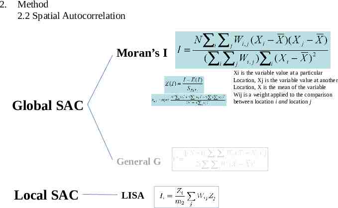
2. Method 2.2 Spatial Autocorrelation Moran’s I Xi is the variable value at a particular Location, Xj is the variable value at another Location, X is the mean of the variable Wij is a weight applied to the comparison between location i and location j Global SAC General G Local SAC LISA
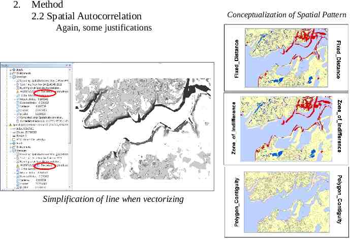
2. Method 2.2 Spatial Autocorrelation Again, some justifications Simplification of line when vectorizing Conceptualization of Spatial Pattern
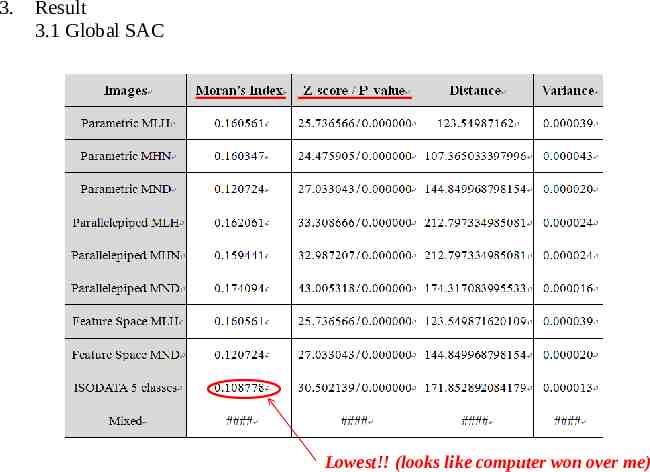
3. Result 3.1 Global SAC Lowest!! (looks like computer won over me)
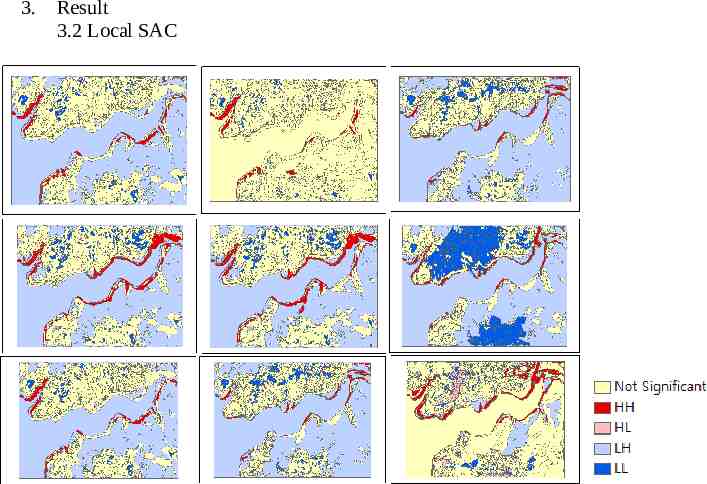
3. Result 3.2 Local SAC
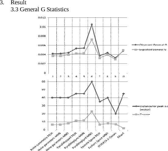
3. Result 3.3 General G Statistics
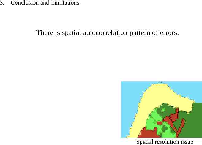
3. Conclusion and Limitations There is spatial autocorrelation pattern of errors. Spatial resolution issue
- Further Plan Also perform initial statistical analysis based on number of pixels for each class Regression analysis (explanatory var: reference image, dependent var: classified image ) Try to look for other classification method (Linear SMA, Fisher linear discriminant etc) Visualization of results (including plotting rook’s, queen’s bishop’s cases) Questions? Suggestions?