Data analytics for Cyber security -Introduction to Data

Data analytics for Cyber security -Introduction to Data MiningVandana P. Janeja 2022 Janeja. All rights reserved.

Outline Knowledge Discovery and Data Mining Process Models Data Preprocessing Data Cleaning Data Transformation and Integration Data Reduction Data Mining Measures of Similarity Measures of Evaluation Clustering Algorithms Classification Pattern Mining: Association Rule Mining Data Analytics for Cybersecurity, 2022 Janeja All rights reserved. 05/08/2024 2

Data Mining Methods Data Analytics for Cybersecurity, 2022 Janeja All rights reserved. 05/08/2024 3

Data Mining methods: Clustering 05/08/2024 Data Analytics for Cybersecurity, 2022 Janeja All rights reserved. 4

Data Mining methods: Clustering Clustering is a technique used for finding similarly behaving groups in data. Should lead to a crisp demarcation of the data such that objects in the same group are highly similar to each other and objects in different groups are very dissimilar to each other Inter cluster distance should be maximized and intra cluster distance should be minimized Clustering helps with the distinction between various types of objects and can be used as an exploratory process and also as a precursor to another mining tasks such as anomaly detection Clustering can be used to identify a structure that could be preexisting in the data Once a cluster is discovered then the objects that are seen outside of this structure could be of interest in some scenarios, or in some other cases the cluster itself could be of interest. For example, if we cluster objects on the basis of certain attributes then some objects which do not conform to the clustering structure could require further investigation as to the cause of this behavior which puts this object outside of the cluster. A cluster of objects could be of interest due to their affinity to each other in some attribute values. Thus, clustering not only can act as an independent analytics approach but in many cases can also be seen as a precursor to other approaches such as outlier detection. Data Analytics for Cybersecurity, 2022 Janeja All rights reserved. 05/08/2024 5

Categorization of the various Clustering approaches Data Analytics for Cybersecurity, 2022 Janeja All rights reserved. 05/08/2024 6

The primary approach of the partitioning algorithms, such as Kmeans, is to form subgroups of the entire set of data, by making K partitions, based on a similarity criterion. The data in the subgroups is grouped around central object such as mean or medoid. However, they differ the way in which they define the similarity criterion, central object and convergence of clusters. K-means (MacQueen 67) Based on finding partitions in the data by evaluating the distance of objects in the cluster to the centroid, which is the mean of the data in the cluster Intuitively the bigger the error the more spread out the points are around the mean If we plot the SSE for K 1 to K n (n number of points), then SSE ranges from a very large value (all points in one cluster) to 0 (every point in its own cluster). The elbow of this plot provides an ideal value of K K-means has been a well-used and well accepted clustering algorithm due to its intuitive approach and interpretable output. However, K-means does not work very well in presence of outliers and does not form non-spherical or free form clusters Partitioning Algorithms: K-means 05/08/2024 Data Analytics for Cybersecurity, 2022 Janeja All rights reserved. 7

Initial seeds, K 2 Clusters K-means clustering Reassignment of Points Starts with a set of points, K value for number of clusters to form and seed centroids which can be selected from the data or randomly generated Partitioning points around the seed centroids such that the point is allocated to the centroid to which its distance is smallest At the end of the first round we have K clusters partitioned around the seed centroids Now the means or centroids of the newly formed clusters are computed and the process is repeated to align the points to the newly computed centroids This process is iterated until there is no more reassignment of the points moving from one cluster to the other K-means works on a heuristic-based partitioning rather than an optimal partitioning The quality of clusters can be evaluated using Sum of squared errors which computes the distance of every point in the cluster to its centroid Centroids recomputed Cluster assignments Clusters No more Reassignment 05/08/2024 Data Analytics for Cybersecurity, 2022 Janeja All rights reserved. 8

Density-Based Algorithm for Discovering Clusters in Large Spatial Databases with Noise, proposed by Ester et. Al. 1996 Foundation of several other density based clustering algorithms Density Based Algorithms: DBSCAN Clusters as dense or sparse regions based on the number of points in the neighborhood region of a point under consideration Radius and a minimum number of points in the region (parameters: , MinPts) Minimum number of points in a radius of facilitates the measurement of density in that neighborhood Neighborhood (in Euclidean point space), is the neighborhood of a point that contains the (minPts) points Variations of DBSCAN also discuss how to identify through computing K distance for every point i.e. if k 2, the distance between the point and its 2nd nearest neighbor, sort this in descending order The K-Distance is plotted and a valley or dip in the K-Distance plot along with a user input of the expected noise determines the neighborhood. The algorithm defines density in terms of core points A Core point is an object, which has the minimum points in its neighborhood defined by Data Analytics for Cybersecurity, 2022 Janeja All rights reserved. 05/08/2024 9

DBSCAN p10 p1 p6 p4 p7 p2 (a) p3 p8 p5 Example: MinPts 3, 1 (b) Core Points: p2, p4, p6, and p7 p1 is Directly Density reachable from p2 p3 is Directly Density reachable from p4 p5 is Directly Density reachable from p6 p6 is Directly Density reachable from p7 p9 p8 is indirectly density reachable from p7 as p8 DDR from p6 and p6 DDR from p7 so by transitivity p8 indirectly density reachable from p7. p1, p3, p5 are all Density connected points. p10 is outlier The DBSCAN algorithm begins by identifying core points and forming clusters through directly density reachable points from this core point. It then merges the cluster with such points. The process terminates when no new point can be added. 05/08/2024 Data Analytics for Cybersecurity, 2022 Janeja All rights reserved. 10

Data Mining methods: Classification 05/08/2024 Data Analytics for Cybersecurity, 2022 Janeja All rights reserved. 11

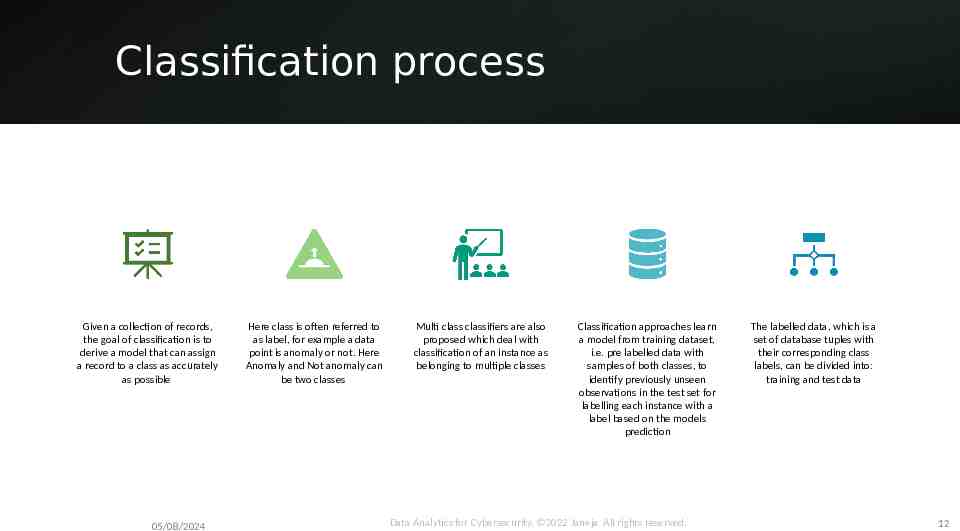
Classification process Given a collection of records, the goal of classification is to derive a model that can assign a record to a class as accurately as possible 05/08/2024 Here class is often referred to as label, for example a data point is anomaly or not. Here Anomaly and Not anomaly can be two classes Multi class classifiers are also proposed which deal with classification of an instance as belonging to multiple classes Classification approaches learn a model from training dataset, i.e. pre labelled data with samples of both classes, to identify previously unseen observations in the test set for labelling each instance with a label based on the models prediction Data Analytics for Cybersecurity, 2022 Janeja All rights reserved. The labelled data, which is a set of database tuples with their corresponding class labels, can be divided into: training and test data 12

Classification process In the training phase, a classification algorithm builds a classifier (set of rules) that learns from a training set Labelled Data This classification model includes some descriptions (rules) for each class using features or attributes in the data Training Data This model is used to determine the class to which a test data instance belongs Classification Model Generation Expert systems 05/08/2024 Accuracy Metrics Test Data In the testing phase, a set of data tuples that are not overlapping with the training tuples are selected. Each test tuple is compared with the classification rules to determine its class The labels of the test tuples are reported along with percentage of correctly classified labels to evaluate the accuracy of the model in previously unseen (labels in the) data Real time Prediction As the model accuracy is evaluated and rules are perfected for labelling previously unseen instances, these rules can be used for future predictions One way to do that is to maintain a knowledge base or expert system with these discovered rules and as incoming data is observed to match these rules the labels for them are predicted. Data Analytics for Cybersecurity, 2022 Janeja All rights reserved. 13

Data Mining methods: Classification Several classification algorithms have been proposed which approach the classification modelling using different mechanisms. The decision tree algorithms provide a set of rules in the form of a decision tree to provide labels based on conditions in the tree branches Bayesian models provide a probability value of an instance belonging to a class Function based methods provide functions for demarcations in the data such that the data is clearly divided between classes Classification combinations namely ensemble methods which combine the classifiers across multiple samples of the training data These methods are designed to increase the accuracy of the classification task by training several different classifiers and combining their results to output a class label A good analogy is when humans seek the input of several experts before making an important decision Diversity among classifier models is a required condition for having a good ensemble classifier (He & Garcia, 2009; Li, 2007) Base classifier in the ensemble should be a weak learner in order to get the best results out of an ensemble A classification algorithm is called a weak learner if a small change in the training data produces big difference in the induced classifier mapping 05/08/2024 Data Analytics for Cybersecurity, 2022 Janeja All rights reserved. 14

Classificat ion Algorithm s 05/08/2024 Data Analytics for Cybersecurity, 2022 Janeja All rights reserved. 15

C4.5 decision tree algorithm starts by evaluating attributes to identify the attribute which gives most information for making a decision for labelling with the class The decision tree provides a series of rules to identify which attribute should be evaluated to come up with the label for a record where the label is unknown These rules form the branches in the decision tree The purity of the attributes to make a decision split in the tree is computed using measures such as Entropy The entropy of a particular node, InfoA (corresponding to an attribute) in a tree is the sum, over all classes represented in the node, of the proportion of records belonging to a particular class Decision Tree Based Classifier: C4.5 05/08/2024 When Entropy reduction is chosen as a splitting criterion, the algorithm searches for the split that reduces entropy or equivalently the split that increases information, learnt from that attribute, by the greatest amount If a leaf in a decision tree is entirely pure then classes in the leaf can be clearly described, that is, they all fall in the same class If a leaf is highly impure then describing it is much more complex Entropy helps us quantify the concept of purity of the node The best split is one that does the best job of separating the records into groups where a single class predominates the group of records in that branch. Data Analytics for Cybersecurity, 2022 Janeja All rights reserved. 16

Example C4.5 ID 1 2 3 4 5 6 7 8 9 10 11 12 13 14 15 16 17 18 (a) DOW Weekday Weekday Weekday Weekday Weekday Weekday Weekday Weekend Weekend Weekend Weekend Weekend Weekend Weekend Weekend Weekend Weekday Weekday packets Flows Attack 400 10K N 400 10K N 400 10K N 400 10K N 400 10K Y 400K& 1000K 10K N 400K& 1000K 10K& 30KN 400K& 1000K 10K& 30KY 1000K 10K& 30KN 1000K 10K& 30KY 1000K 10K& 30KY 1000K 10K& 30KN 1000K 10K& 30KN 1000K 30K Y 1000K 30K Y 1000K 30K Y 1000K 30K Y 400K& 1000K 30K N DOW Weekday Weekend Attack Y 2 Attack N 7 packets 400 Attack Y Attack N Flows 10k Attack Y Attack N (b) 6 3 400K& 1000K 1000 1 1 4 3 10K& 30K 1 5 6 3 30K 3 4 4 1 Info(D) Info(Packets) Info(Flows) Info (DOW) 0.99 0.84 0.80 0.84 (d) 10K N Flows 10K& 30K N 30K Y Gain Packets Flows 0.15 DOW 0.19 (c) 0.15

Entropy computation for data set and attributes Expected information needed to classify a tuple in a Dataset How much more info would you still need (after partitioning) to get exact classification? How much would be gained by partitioning on this attribute? Expected reduction in the information requirement caused by knowing the

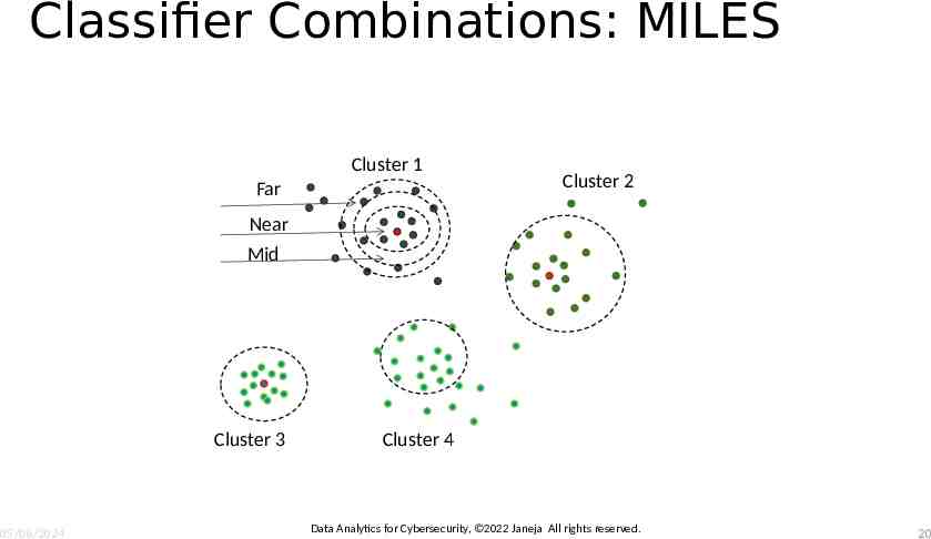
Classifier Combinatio nsEnsemble Method: MILES In ensemble learning, it is important to form learning sets from different regions in the feature space. Particularly important if the data is imbalanced and has distribution of multiple classes with some majority and minority classes in the feature space Learning sets that are dissimilar can produce more diverse results Multiclass Imbalanced Learning in Ensembles through Selective Sampling (MILES) Creates training sets using clustering-based selective sampling Uses k cluster sets to selectively choose the training samples MILES adopts clustering as a stratified sampling approach to form a set of learning sets that are different from each other and at the same time each one of them is representative of the original learning set D Rebalances the training sets Utilizes the concept of split ratio (SR) to split the examples in clusters into three strata (near, far and mid) around the cluster centroids Combines the classifiers and forming the ensemble Data Analytics for Cybersecurity, 2022 Janeja All rights reserved. 05/08/2024 19

Classifier Combinations: MILES Cluster 1 Far Cluster 2 Near Mid Cluster 3 05/08/2024 Cluster 4 Data Analytics for Cybersecurity, 2022 Janeja All rights reserved. 20

Data Mining methods: Pattern Mining 05/08/2024 Data Analytics for Cybersecurity, 2022 Janeja All rights reserved. 21

Data Mining methods: Pattern Mining Pattern refers to occurrence of multiple objects in a certain combination, which could lead to discovery of an implicit interaction A frequent pattern refers to frequently co-occurring objects A rare pattern refers to a combination of objects not normally occurring and which could lead to identification of a possible unusual interaction between the objects Events become relevant when they occur together in a sequence or as groups Some approaches deal with this as a causal problem and therefore rely on conditional probability of events to determine the occurrence If events are seen as itemsets in transactions, focus has been put on finding conditional relationships such that presence of A causes B with a certain probability There might be events where there might be no implied causal relationships between them but the relationship is based purely on co-occurrence For example events might have no implied or evident causal relationship but a co-occurrence relationship based on frequency of occurrence based on a certain degree of support or confidence defining the probability of one event given the other Data Analytics for Cybersecurity, 2022 Janeja All rights reserved. 05/08/2024 22

Categorization of the various pattern mining approaches 05/08/2024 Data Analytics for Cybersecurity, 2022 Janeja All rights reserved. 23

Frequent Pattern Mining: Apriori The Apriori algorithm is based on finding frequent itemsets and then discovering and quantifying the association rules It provides efficient mechanism of discovering frequent item sets A subset of a frequent itemset must also be a frequent itemset i.e., if {IP1, high} is a frequent itemset, both {IP1} and {high} should be a frequent itemset It iteratively finds frequent itemsets with cardinality from 1 to k (k-itemset). It uses the frequent itemsets to generate association rules The apriori generates the candidate itemsets by joining the itemsets with large support from the previous pass and deleting the subsets, which have small support from the previous pass By only considering the itemsets with large support, the number of candidate itemsets is significantly reduced. In the first pass itemsets with only one item are counted The itemsets with higher support are used to generate the candidate sets of the second pass Once the candidate itemsets are found, their supports are calculated to discover the items sets of size two with large support and so on This process terminates when no new itemsets are found with large support Here min support is predetermined as a user defined threshold A confidence threshold is predetermined by the user Data Analytics for Cybersecurity, 2022 Janeja All rights reserved. 05/08/2024 24

Example : Apriori Algorithm min supp 2 t1 IP1 t2 IP2 t3 IP1 t4 IP4 t5 IP4 t6 IP6 t7 IP1 t8 IP6 high high high low low high high med Candidate set 1 IP1 IP2 IP4 IP6 high med low A set of transactions containing IP addresses and level of alerts raised in an IDS (high, med and low) If IP1 and high are two items the association rule IP1 high means that whenever an item IP1 occurs in a transaction then high also occurs with a quantified probability The probability or confidence threshold can be defined as the percentage of transactions containing high and IP1 with respect to the percentage of transactions containing just IP1 This can be seen in terms of conditional probability where P (high IP1) P (IP1 U high) / P (IP1). The strength of the rule can also be quantified in terms of support, where support is the number of transactions, which contain a certain item, therefore support of X is the percentage of transactions containing X in the entire set of transactions. Confidence is determined as Support (IP1 U high) / Support (IP1) This gives the confidence and support for rule for IP1 high The rule IP1 high is not the same as high IP1 as the confidence will change IP1 high high IP1 IP4 low low IP4 05/08/2024 Confidence IP1& high/ IP1 IP1& high/ high IP4&low/IP4 IP4 & low/low 1 0.6 1 1 Support IP1& high/ # tuples IP1& high/ # tuples IP4&low/ # tuples IP4 & low/ # tuples Data Analytics for Cybersecurity, 2022 Janeja All rights reserved. Frequent item set IP1 IP4 IP6 high low 3 1 2 2 5 1 2 1 3 2 2 5 3 Candidate set 2 IP1, IP4 IP1, high IP1, low IP4, high IP4, low IP6, low IP6, med IP6, high high, low 0.38 0.38 0.25 0.25 0 3 0 0 2 0 1 1 0 Frequent item set 2 IP1, high 3 IP4, low 2 25

Selected References Fayyad, Usama, Gregory Piatetsky-Shapiro, and Padhraic Smyth. "From data mining to knowledge discovery in databases." AI magazine 17.3 (1996): 37. Shearer C., The CRISP-DM model: the new blueprint for data mining, J Data Warehousing (2000); 5:13—22. Pete Chapman (NCR), Julian Clinton (SPSS), Randy Kerber (NCR), Thomas Khabaza (SPSS), Thomas Reinartz (DaimlerChrysler), Colin Shearer (SPSS) and Rüdiger Wirth (DaimlerChrysler), CRISP-DM 1.0 , Step-by-Step data mining guide, 2000 Lukasz A. Kurgan and Petr Musilek. 2006. A survey of Knowledge Discovery and Data Mining process models. Knowl. Eng. Rev. 21, 1 (March 2006), 1-24. DOI http://dx.doi.org/10.1017/S0269888906000737 Famili, A., Shen, W. M., Weber, R., & Simoudis, E. (1997). Data preprocessing and intelligent data analysis. Intelligent data analysis, 1(1-4), 3-23. Liu, H., Hussain, F., Tan, C. L., & Dash, M. (2002). Discretization: An enabling technique. Data mining and knowledge discovery, 6(4), 393-423. Garcia, S., Luengo, J., Sáez, J. A., Lopez, V., & Herrera, F. (2013). A survey of discretization techniques: Taxonomy and empirical analysis in supervised learning. IEEE Transactions on Knowledge and Data Engineering, 25(4), 734-750. Al Shalabi, L., Shaaban, Z., & Kasasbeh, B. (2006). Data mining: A preprocessing engine. Journal of Computer Science, 2(9), 735-739. Chandrashekar, G., & Sahin, F. (2014). A survey on feature selection methods. Computers & Electrical Engineering, 40(1), 16-28. Molina, L. C., Belanche, L., & Nebot, À. (2002). Feature selection algorithms: A survey and experimental evaluation. In Data Mining, 2002. ICDM 2003. Proceedings. 2002 IEEE International Conference on (pp. 306-313). IEEE. Fodor, Imola K. "A survey of dimension reduction techniques." Center for Applied Scientific Computing, Lawrence Livermore National Laboratory 9 (2002): 1-18. Wall, M. E., Rechtsteiner, A., & Rocha, L. M. (2003). Singular value decomposition and principal component analysis. In A practical approach to microarray data analysis (pp. 91-109). Springer US. Wu, X., Kumar, V., Quinlan, J. R., Ghosh, J., Yang, Q., Motoda, H., . & Zhou, Z. H. (2008). Top 10 algorithms in data mining. Knowledge and information systems, 14(1), 1-37. Leskovec, J., Kleinberg, J., & Faloutsos, C. (2005, August). Graphs over time: densification laws, shrinking diameters and possible explanations. In Proceedings of the eleventh ACM SIGKDD international conference on Knowledge discovery in data mining (pp. 177-187). ACM. Shashi Shekhar, Chang-tien Lu, Pusheng Zhang, Detecting Graph-based Spatial Outliers: Algorithms and Applications, Proc. of the 7th ACM SIGKDD International Conference on Knowledge Discovery and Data Mining, 2001 Joachims, T. (2002, July). Optimizing search engines using clickthrough data. In Proceedings of the eighth ACM SIGKDD international conference on Knowledge discovery and data mining (pp. 133-142). ACM. Ester, M., Kriegel, H. P., Sander, J., & Xu, X. (1996, August). A density-based algorithm for discovering clusters in large spatial databases with noise. In Kdd (Vol. 96, No. 34, pp. 226-231). Hu, M., & Liu, B. (2004, August). Mining and summarizing customer reviews. In Proceedings of the tenth ACM SIGKDD international conference on Knowledge discovery and data mining (pp. 168-177). ACM. L. Kaufman and P. J. Rousseeuw. Finding Groups in Data: an Introduction to Cluster Analysis. John Wiley & Sons, 1990. MacQueen, J. (1967, June). Some methods for classification and analysis of multivariate observations. In Proceedings of the fifth Berkeley symposium on mathematical statistics and probability (Vol. 1, No. 14, pp. 281-297). 05/08/2024 Data Analytics for Cybersecurity, 2022 Janeja All rights reserved. 26 Kaufman, L., & Rousseeuw, P. (1987). Clustering by means of medoids. North-Holland.

Selected References Ng, R. T., & Han, J. (1994, September). E cient and E ective Clustering Methods for Spatial Data Mining. In Proc. of (pp. 144-155). Zhang, T., Ramakrishnan, R., & Livny, M. (1996, June). BIRCH: an efficient data clustering method for very large databases. In ACM Sigmod Record (Vol. 25, No. 2, pp. 103-114). ACM. Guha, S., Rastogi, R., & Shim, K. (1998, June). CURE: an efficient clustering algorithm for large databases. In ACM Sigmod Record (Vol. 27, No. 2, pp. 73-84). ACM. Karypis, G., Han, E. H., & Kumar, V. (1999). Chameleon: Hierarchical clustering using dynamic modeling. Computer, 32(8), 68-75. Ankerst, M., Breunig, M. M., Kriegel, H. P., & Sander, J. (1999, June). OPTICS: ordering points to identify the clustering structure. In ACM Sigmod record (Vol. 28, No. 2, pp. 49-60). ACM. Hinneburg, A., & Keim, D. A. (1998, August). An efficient approach to clustering in large multimedia databases with noise. In KDD (Vol. 98, pp. 58-65). Sander, J., Ester, M., Kriegel, H. P., & Xu, X. (1998). Density-based clustering in spatial databases: The algorithm gdbscan and its applications. Data mining and knowledge discovery, 2(2), 169-194. Xu, X., Jäger, J., & Kriegel, H. P. (1999). A fast parallel clustering algorithm for large spatial databases. In High Performance Data Mining (pp. 263-290). Springer US. Xu, X., Ester, M., Kriegel, H. P., & Sander, J. (1998, February). A distribution-based clustering algorithm for mining in large spatial databases. In Data Engineering, 1998. Proceedings., 14th International Conference on (pp. 324-331). IEEE. Jarvis, Raymond Austin, and Edward A. Patrick. "Clustering using a similarity measure based on shared near neighbors." IEEE Transactions on computers 100.11 (1973): 1025-1034. Zhou, B., Cheung, D. W., & Kao, B. (1999, April). A fast algorithm for density-based clustering in large database. In Pacific-Asia Conference on Knowledge Discovery and Data Mining (pp. 338-349). Springer Berlin Heidelberg. Stutz, J., & Cheeseman, P. (1996). AutoClass—a Bayesian approach to classification. In Maximum entropy and Bayesian methods (pp. 117-126). Springer Netherlands. Gennari, J. H., Langley, P., & Fisher, D. (1989). Models of incremental concept formation. Artificial intelligence, 40(1-3), 11-61. Dempster, A. P., Laird, N. M., & Rubin, D. B. (1977). Maximum likelihood from incomplete data via the EM algorithm. Journal of the royal statistical society. Series B (methodological), 1-38. Peña, J. M., Lozano, J. A., & Larrañaga, P. (2002). Learning recursive Bayesian multinets for data clustering by means of constructive induction. Machine Learning, 47(1), 63-89. Wang, W., Yang, J., & Muntz, R. (1997, August). STING: A statistical information grid approach to spatial data mining. In VLDB (Vol. 97, pp. 186-195). R. Agrawal, J. Gehrke, D. Gunopulos, and P. Raghavan. Automatic subspace clustering of high dimensional data for data mining applications. In Proceedings of the 1998 ACM SIGMOD international conference on Management of data, pages 94{105. ACM Press, 1998. Guha, S., Rastogi, R., & Shim, K. (2000). ROCK: A robust clustering algorithm for categorical attributes. Information systems, 25(5), 345-366. Peter J. Rousseeuw (1987). "Silhouettes: a Graphical Aid to the Interpretation and Validation of Cluster Analysis". Computational and Applied Mathematics. 20: 53– 65 05/08/2024 Data Analytics for Cybersecurity, 2022 Janeja All rights reserved. 27