Production Theory 2

35 Slides141.00 KB
Production Theory 2
Returns-to-Scale Marginal product describe the change in output level as a single input level changes. (Short-run) Returns-to-scale describes how the output level changes as all input levels change, e.g. all input levels doubled. (Long-run)
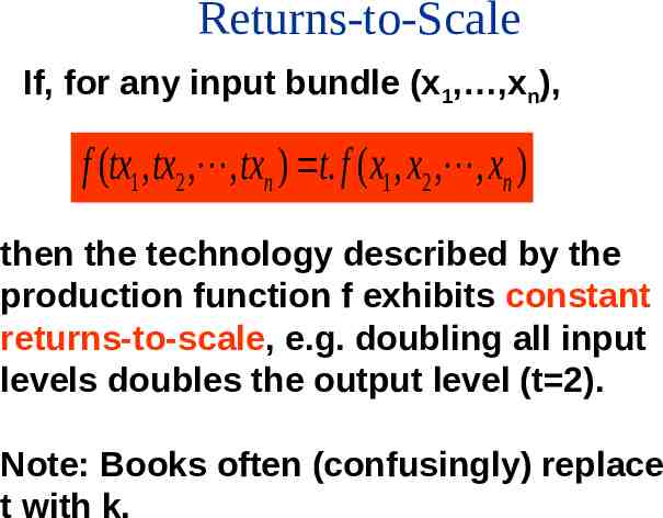
Returns-to-Scale If, for any input bundle (x1, ,xn), f (tx1 , tx2 , , txn ) t. f ( x1 , x2 , , xn ) then the technology described by the production function f exhibits constant returns-to-scale, e.g. doubling all input levels doubles the output level (t 2). Note: Books often (confusingly) replace t with k.
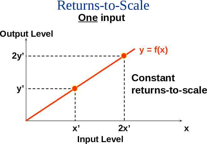
Returns-to-Scale One input Output Level y f(x) 2y’ Constant returns-to-scale y’ x’ 2x’ Input Level x
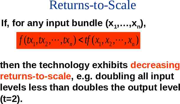
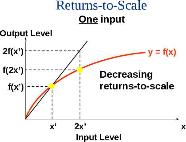
Returns-to-Scale If, for any input bundle (x1, ,xn), f (tx1 , tx2 , , txn ) tf ( x1 , x2 , , xn ) then the technology exhibits decreasing returns-to-scale, e.g. doubling all input levels less than doubles the output level (t 2).
Returns-to-Scale One input Output Level 2f(x’) y f(x) f(2x’) Decreasing returns-to-scale f(x’) x’ 2x’ Input Level x
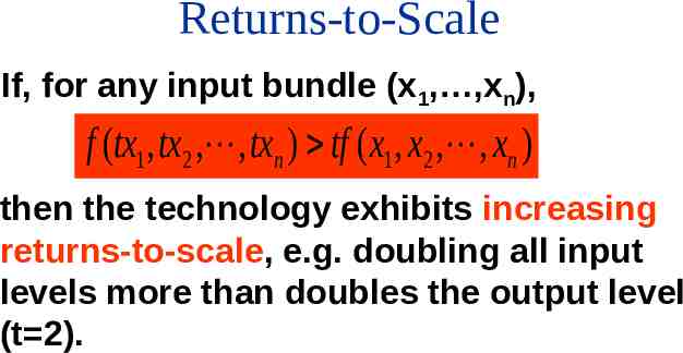
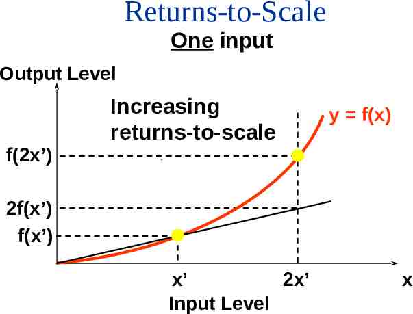
Returns-to-Scale If, for any input bundle (x1, ,xn), f (tx1 , tx2 , , txn ) tf ( x1 , x2 , , xn ) then the technology exhibits increasing returns-to-scale, e.g. doubling all input levels more than doubles the output level (t 2).
Returns-to-Scale One input Output Level f(2x’) Increasing returns-to-scale y f(x) 2f(x’) f(x’) x’ 2x’ Input Level x
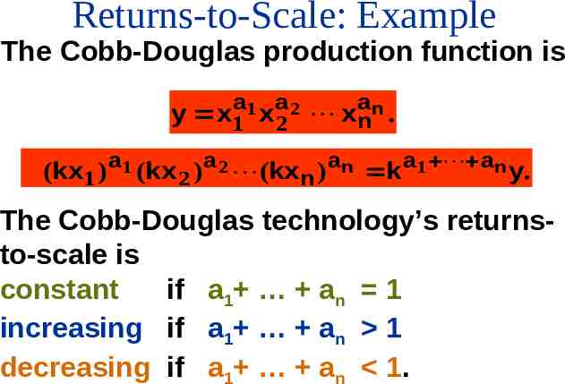
Returns-to-Scale: Example The Cobb-Douglas production function is 2 x an . y x1a1 xa n 2 (kx1 ) a1 (kx 2 ) a 2 (kxn ) an ka1 an y. The Cobb-Douglas technology’s returnsto-scale is constant if a1 an 1 increasing if a1 an 1 decreasing if a1 an 1.
Short-Run: Marginal Product A marginal product is the rate-ofchange of output as one input level increases, holding all other input levels fixed. Marginal product diminishes because the other input levels are fixed, so the increasing input’s units each have less and less of other inputs with which to work.
Long-Run: Returns-to-Scale When all input levels are increased proportionately, there need be no such “crowding out” as each input will always have the same amount of other inputs with which to work. Input productivities need not fall and so returns-to-scale can be constant or even increasing.
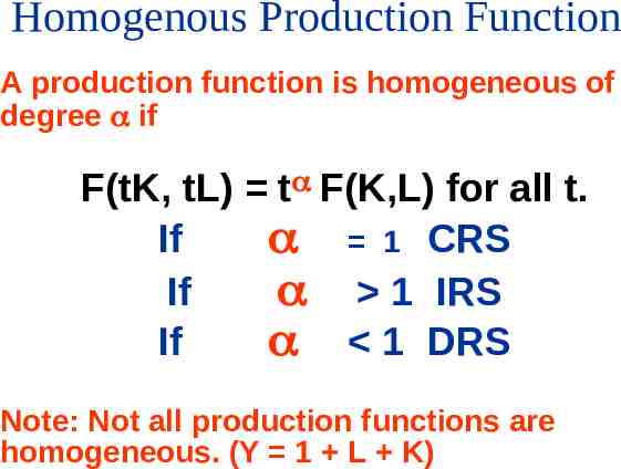
Homogenous Production Function A production function is homogeneous of degree if F(tK, tL) t F(K,L) for all t. If 1 CRS If 1 IRS If 1 DRS Note: Not all production functions are homogeneous. (Y 1 L K)
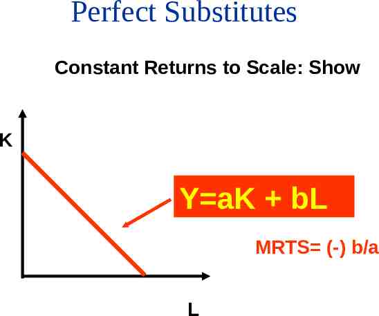
Perfect Substitutes Constant Returns to Scale: Show K Y aK bL MRTS (-) b/a L
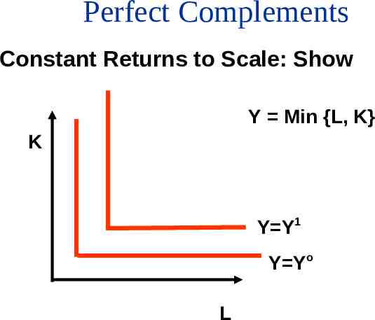
Perfect Complements Constant Returns to Scale: Show Y Min {L, K} K Y Y1 Y Yo L
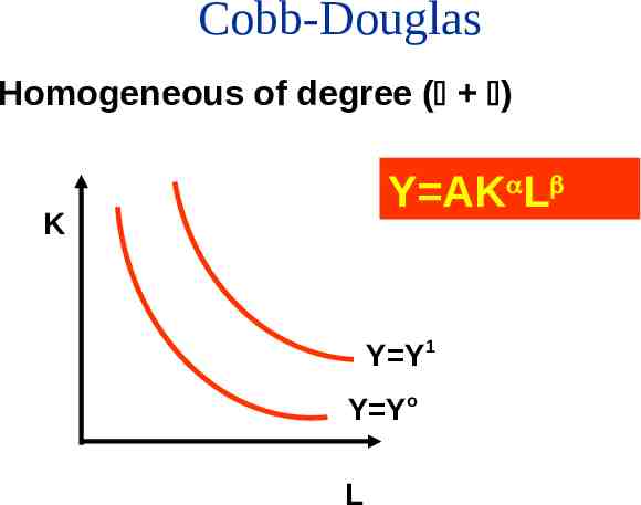
Cobb-Douglas Homogeneous of degree ( ) Y AK L K Y Y1 Y Yo L
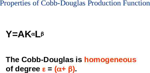
Properties of Cobb-Douglas Production Function Y AK L The Cobb-Douglas is homogeneous of degree ( ).
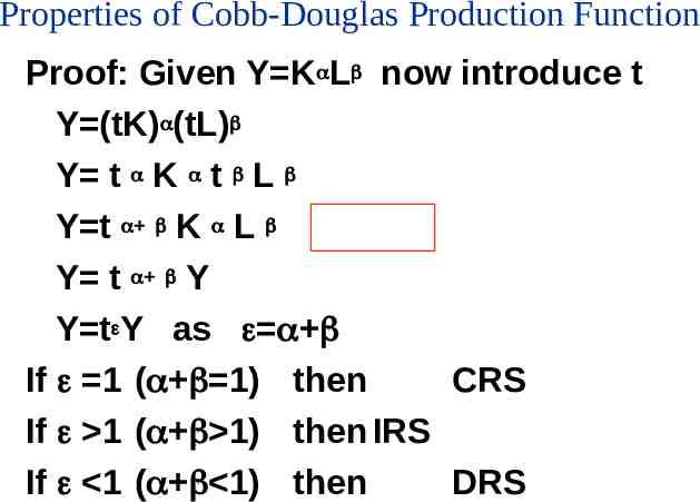
Properties of Cobb-Douglas Production Function Proof: Given Y K L now introduce t Y (tK) (tL) Y t K t L Y t K L Y t Y Y t Y as If 1 ( 1) then CRS If 1 ( 1) then IRS If 1 ( 1) then DRS
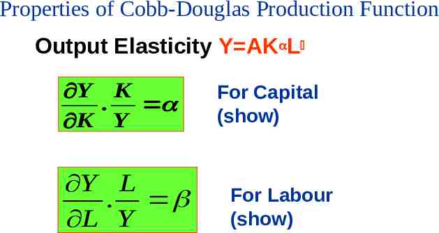
Properties of Cobb-Douglas Production Function Output Elasticity Y AK L Y K . K Y Y L . L Y For Capital (show) For Labour (show)
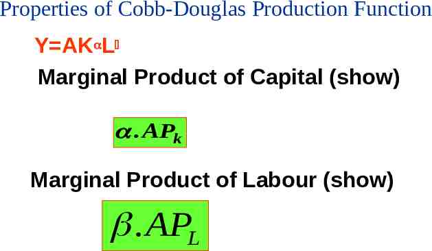
Properties of Cobb-Douglas Production Function Y AK L Marginal Product of Capital (show) . APk Marginal Product of Labour (show) . APL
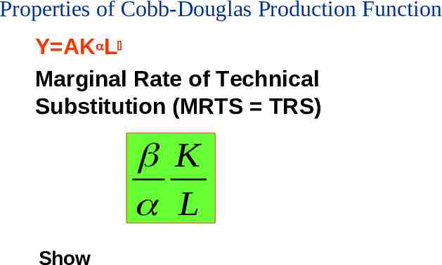
Properties of Cobb-Douglas Production Function Y AK L Marginal Rate of Technical Substitution (MRTS TRS) K L Show
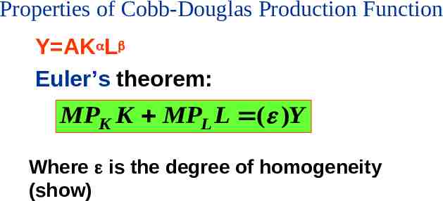
Properties of Cobb-Douglas Production Function Y AK L Euler’s theorem: MPK K MPL L ( )Y Where is the degree of homogeneity (show)
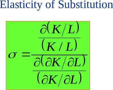
Elasticity of Substitution The Elasticity of Substitution is the ratio of the proportionate change in factor proportions to the proportionate change in the slope of the isoquant. Intuition: If a small change in the slope of the isoquant leads to a large change in the K/L ratio then capital and labour are highly substitutable.
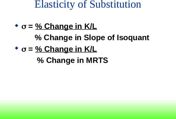
Elasticity of Substitution % Change in K/L % Change in Slope of Isoquant % Change in K/L % Change in MRTS
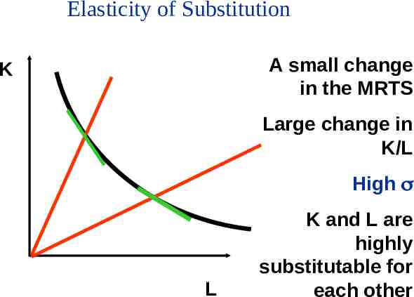
Elasticity of Substitution A small change in the MRTS K Large change in K/L High L K and L are highly substitutable for each other
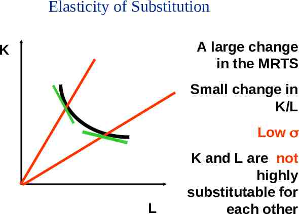
Elasticity of Substitution A large change in the MRTS K Small change in K/L Low L K and L are not highly substitutable for each other
Elasticity of Substitution K L K / L K L K L
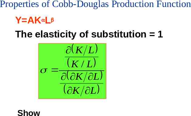
Properties of Cobb-Douglas Production Function Y AK L The elasticity of substitution 1 K L K / L K L K L Show
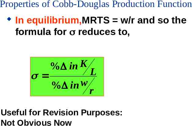
Properties of Cobb-Douglas Production Function In equilibrium,MRTS w/r and so the formula for reduces to, % in K % in w L r Useful for Revision Purposes: Not Obvious Now
Properties of Cobb-Douglas Production Function For the Cobb-Douglas, 1 means that a 10% change in the factor price ratio leads to a 10% change in the opposite direction in the factor input ratio. Useful For Revision Purposes: Not Obvious Now
Well-Behaved Technologies A well-behaved technology is – monotonic, and – convex.
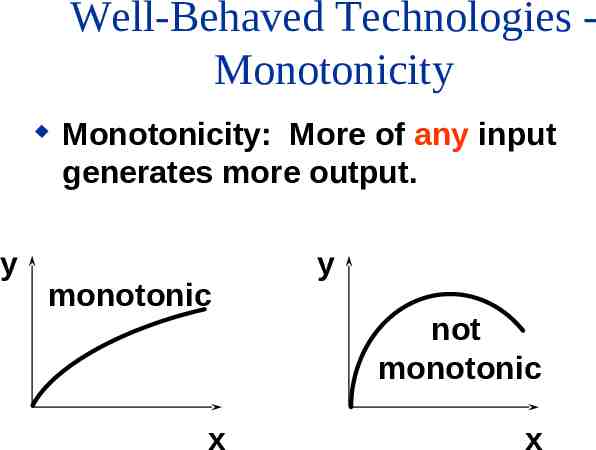
Well-Behaved Technologies Monotonicity y Monotonicity: More of any input generates more output. monotonic x y not monotonic x
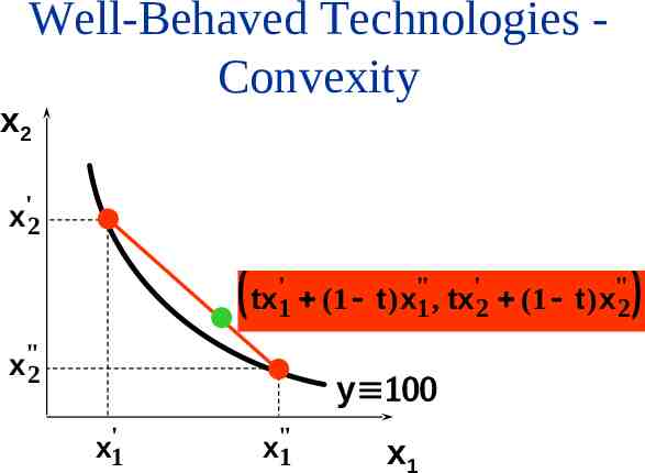
Well-Behaved Technologies Convexity Convexity: If the input bundles x’ and x” both provide y units of output then the mixture tx’ (1-t)x” provides at least y units of output, for any 0 t 1.
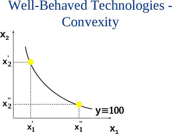
Well-Behaved Technologies Convexity x2 ' x2 x"2 y x'1 x"1 x1
Well-Behaved Technologies Convexity x2 ' x2 tx'1 (1 t )x"1 , tx'2 (1 t )x"2 x"2 y x'1 x"1 x1
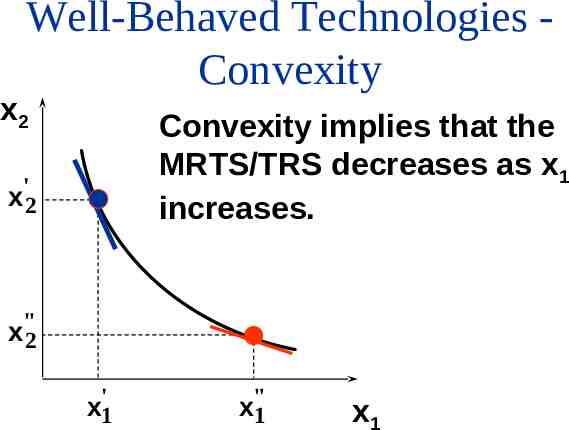
Well-Behaved Technologies Convexity x2 Convexity implies that the MRTS/TRS decreases as x1 increases. ' x2 x"2 x'1 x"1 x1