Practical Statistical Analysis Objectives: Conceptually understand the

Practical Statistical Analysis Objectives: Conceptually understand the following for both linear and nonlinear models: 1. Best fit to model parameters 2. Experimental error and its estimate 3. Prediction confidence bands 4. Single-point confidence bands 5. Parameter confidence regions 6. Experimental design

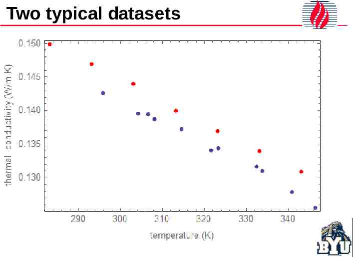
Two typical datasets

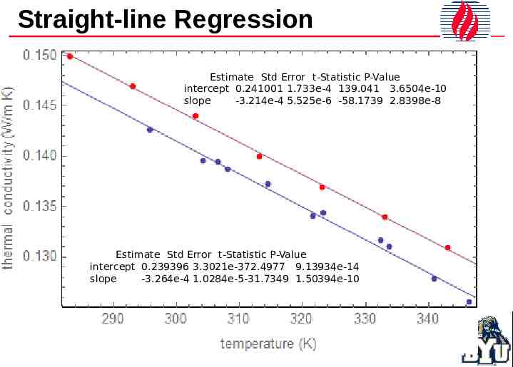
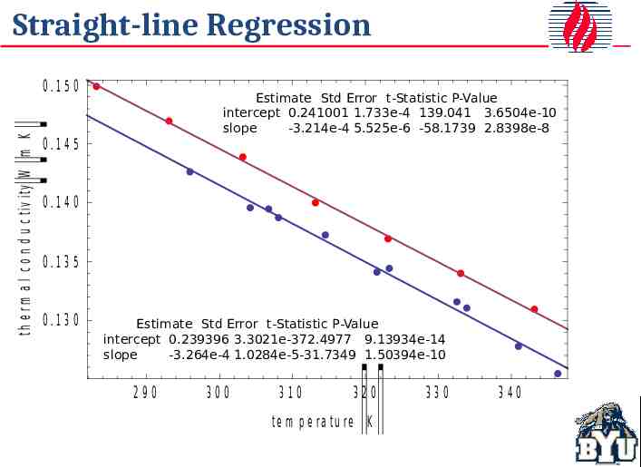
Straight-line Regression Estimate Std Error t-Statistic P-Value intercept 0.241001 1.733e-4 139.041 3.6504e-10 slope -3.214e-4 5.525e-6 -58.1739 2.8398e-8 Estimate Std Error t-Statistic P-Value intercept 0.239396 3.3021e-372.4977 9.13934e-14 slope -3.264e-4 1.0284e-5-31.7349 1.50394e-10

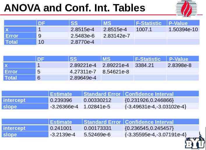
ANOVA and Conf. Int. Tables x Error Total DF 1 9 10 SS 2.8515e-4 2.5483e-6 2.8770e-4 MS 2.8515e-4 2.83142e-7 F-Statistic 1007.1 P-Value 1.50394e-10 x Error Total DF 1 5 6 SS 2.89221e-4 4.27311e-7 2.89649e-4 MS 2.89221e-4 8.54621e-8 F-Statistic 3384.21 P-Value 2.8398e-8 intercept slope Estimate 0.239396 -3.26366e-4 Standard Error Confidence Interval 0.00330212 {0.231926,0.246866} 1.02841e-5 {-3.49631e-4,-3.03102e-4} intercept slope Estimate 0.241001 -3.2139e-4 Standard Error Confidence Interval 0.00173331 {0.236545,0.245457} 5.52469e-6 {-3.35595e-4,-3.07191e-4}

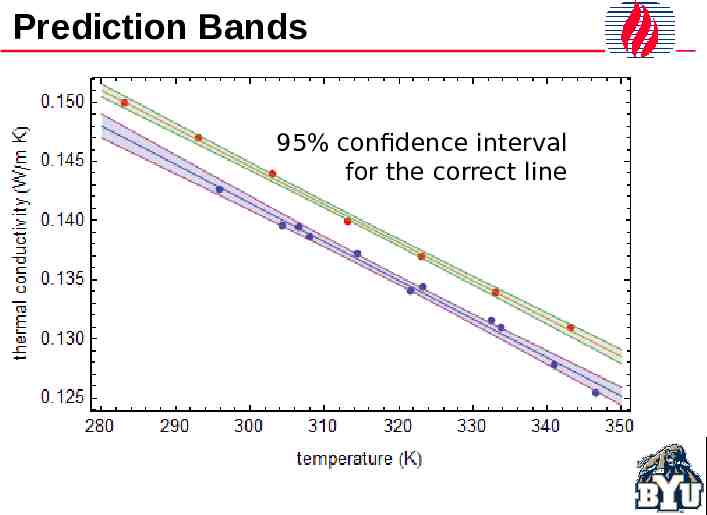
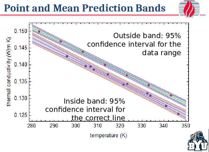
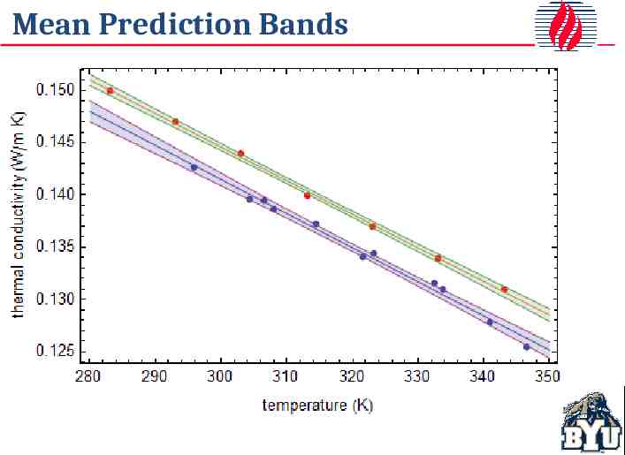
Prediction Bands 95% confidence interval for the correct line

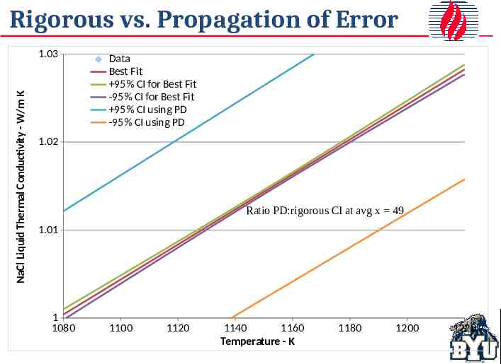
Propagation of Error

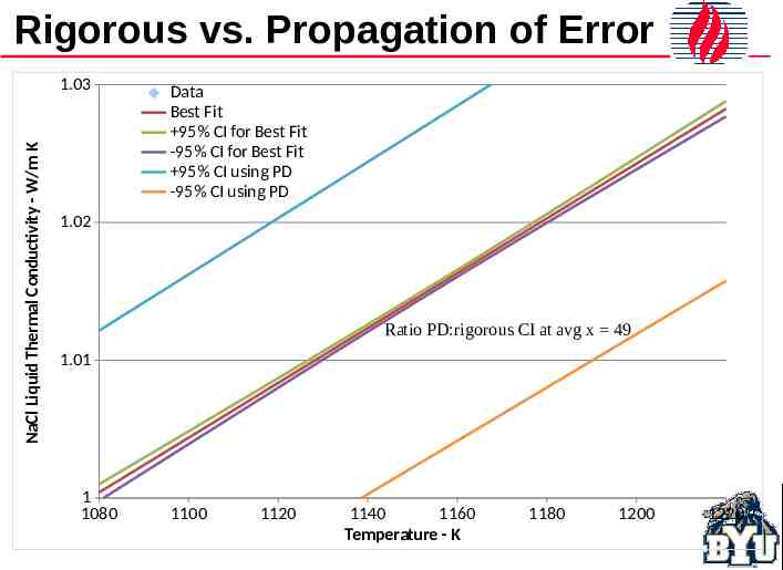
Rigorous vs. Propagation of Error NaCl Liquid Thermal Conductivity - W/m K 1.03 Data Best Fit 95% CI for Best Fit -95% CI for Best Fit 95% CI using PD -95% CI using PD 1.02 Ratio PD:rigorous CI at avg x 49 1.01 1 1080 1100 1120 1140 1160 Temperature - K 1180 1200 1220

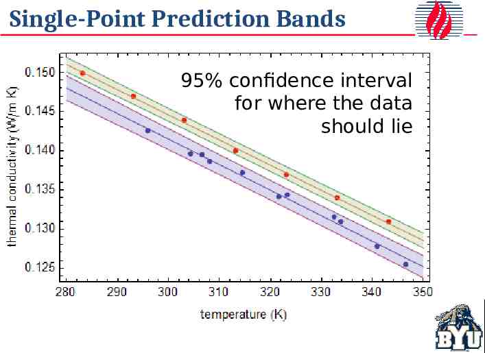
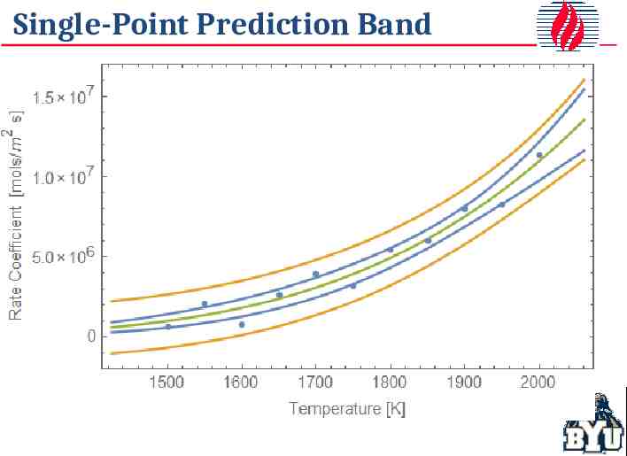
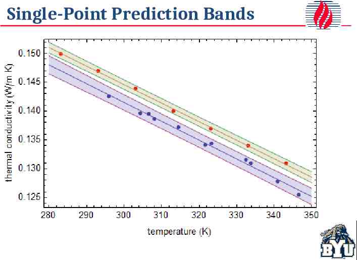
Single-Point Prediction Bands 95% confidence interval for where the data should lie

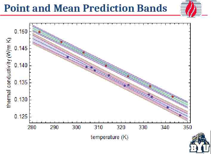
Point and Mean Prediction Bands Outside band: 95% confidence interval for the data range Inside band: 95% confidence interval for the correct line

Confidence Interval Ranges

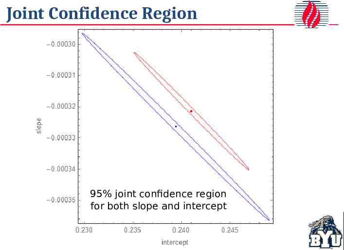
Joint Confidence Region 95% joint confidence region for both slope and intercept

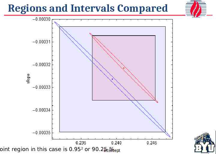
Regions and Intervals Compared oint region in this case is 0.952 or 90.25 %

Single-Point Prediction Band

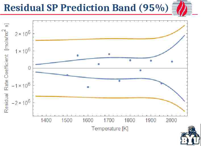
Residual SP Prediction Band (95%)

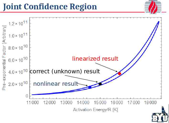
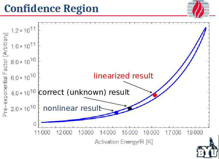
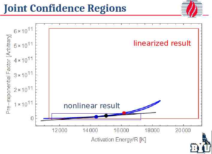
Joint Confidence Region linearized result correct (unknown) result nonlinear result

Joint Confidence Regions linearized result nonlinear result

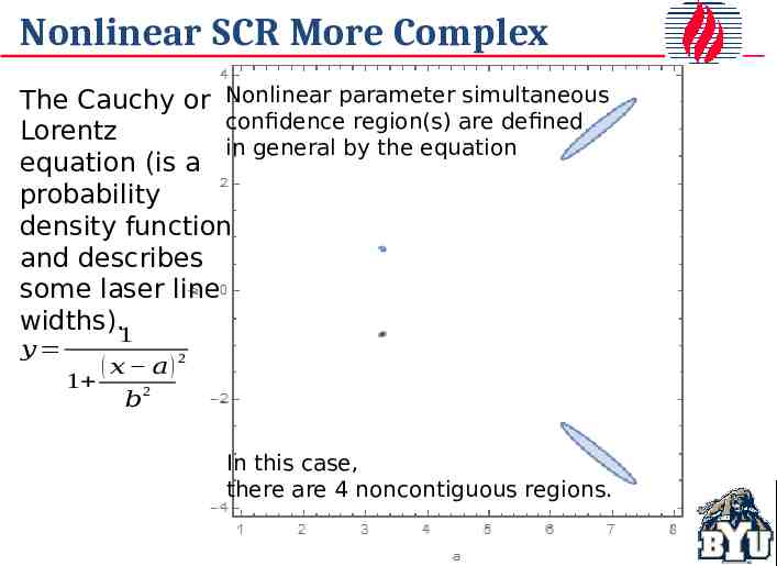
Nonlinear SCR More Complex The Cauchy or Nonlinear parameter simultaneous confidence region(s) are defined Lorentz in general by the equation equation (is a probability density function and describes some laser line widths).1 𝑦 ( 𝑥 𝑎)2 1 2 𝑏 In this case, there are 4 noncontiguous regions.

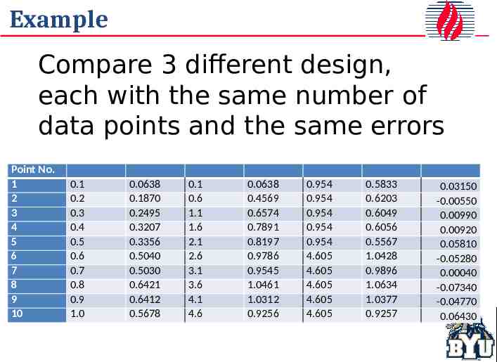
Example Compare 3 different design, each with the same number of data points and the same errors Point No. 1 2 3 4 5 6 7 8 9 10 0.1 0.2 0.3 0.4 0.5 0.6 0.7 0.8 0.9 1.0 0.0638 0.1870 0.2495 0.3207 0.3356 0.5040 0.5030 0.6421 0.6412 0.5678 0.1 0.6 1.1 1.6 2.1 2.6 3.1 3.6 4.1 4.6 0.0638 0.4569 0.6574 0.7891 0.8197 0.9786 0.9545 1.0461 1.0312 0.9256 0.954 0.954 0.954 0.954 0.954 4.605 4.605 4.605 4.605 4.605 0.5833 0.6203 0.6049 0.6056 0.5567 1.0428 0.9896 1.0634 1.0377 0.9257 0.03150 -0.00550 0.00990 0.00920 0.05810 -0.05280 0.00040 -0.07340 -0.04770 0.06430

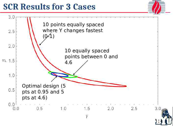
SCR Results for 3 Cases 10 points equally spaced where Y changes fastest (0-1) 10 equally spaced points between 0 and 4.6 Optimal design (5 pts at 0.95 and 5 pts at 4.6)

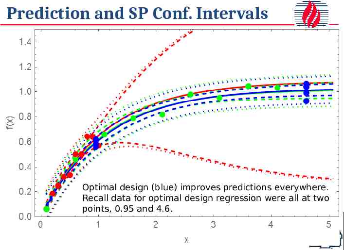
Prediction and SP Conf. Intervals Optimal design (blue) improves predictions everywhere. Recall data for optimal design regression were all at two points, 0.95 and 4.6.

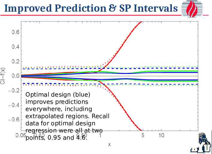
Improved Prediction & SP Intervals Optimal design (blue) improves predictions everywhere, including extrapolated regions. Recall data for optimal design regression were all at two points, 0.95 and 4.6.

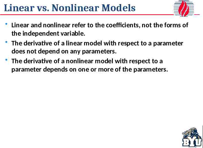
Linear vs. Nonlinear Models Linear and nonlinear refer to the coefficients, not the forms of the independent variable. The derivative of a linear model with respect to a parameter does not depend on any parameters. The derivative of a nonlinear model with respect to a parameter depends on one or more of the parameters.

Linear vs. Nonlinear Models Linear Models Nonlinear Models in general no general expression

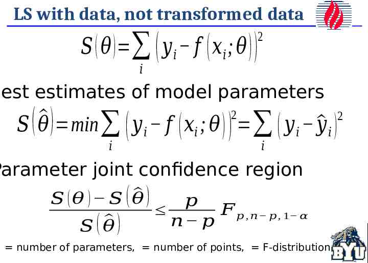
LS with data, not transformed data 2 𝑆 ( 𝜃 ) ( 𝑦 𝑖 𝑓 ( 𝑥 𝑖 ; 𝜃 ) ) 𝑖 Best estimates of model parameters 2 2 𝑆 ( 𝜃 ) min ( 𝑦 𝑖 𝑓 ( 𝑥𝑖 ; 𝜃 ) ) ( 𝑦 𝑖 𝑦 𝑖 ) 𝑖 𝑖 Parameter joint confidence region ) 𝑆 (𝜃 ) 𝑆 ( 𝜃 𝑝 𝐹 𝑝 ,𝑛 𝑝 , 1 𝛼 ) 𝑛 𝑝 𝑆(𝜃 number of parameters, number of points, F-distribution

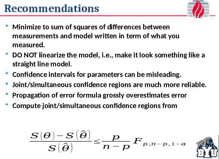
Recommendations Minimize to sum of squares of differences between measurements and model written in term of what you measured. DO NOT linearize the model, i.e., make it look something like a straight line model. Confidence intervals for parameters can be misleading. Joint/simultaneous confidence regions are much more reliable. Propagation of error formula grossly overestimates error Compute joint/simultaneous confidence regions from ) 𝑆 (𝜃 ) 𝑆 ( 𝜃 𝑝 𝐹 𝑝 , 𝑛 𝑝 , 1 𝛼 ) 𝑛 𝑝 𝑆(𝜃

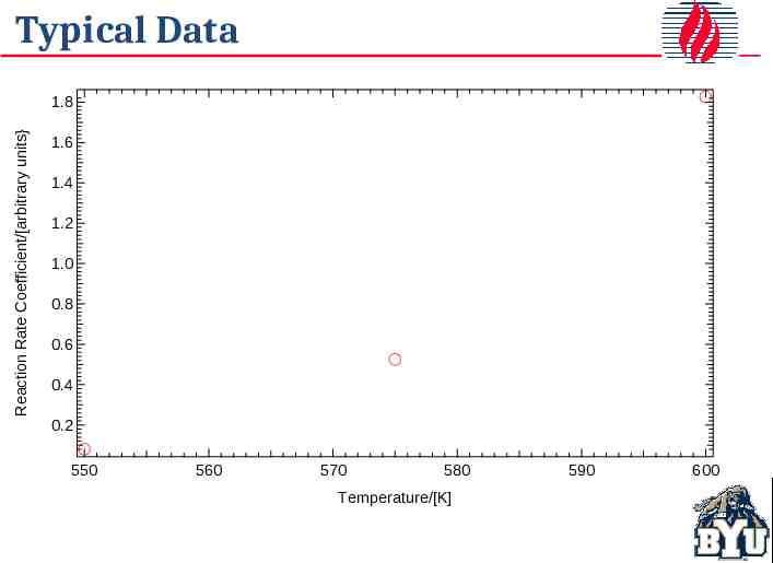
Typical Data Reaction Rate Coefficient/[arbitrary units} 1.8 1.6 1.4 1.2 1.0 0.8 0.6 0.4 0.2 550 560 570 580 Temperature/[K] 590 600

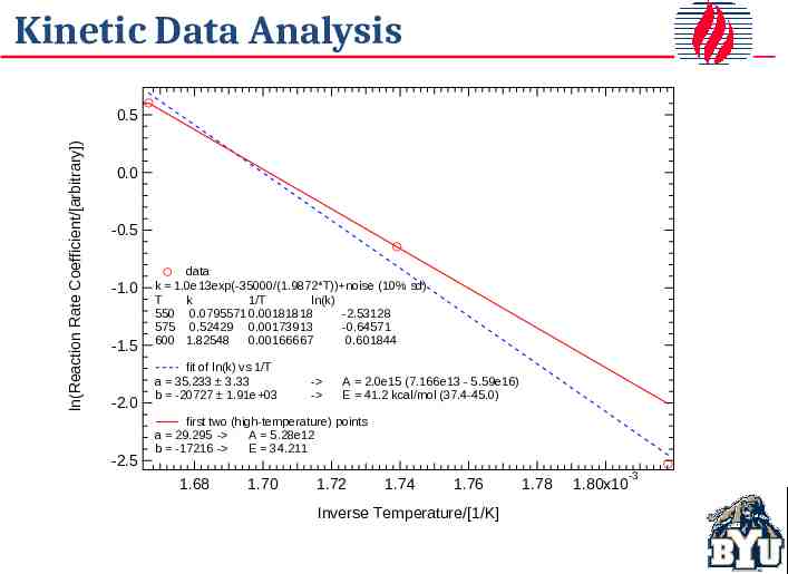
Kinetic Data Analysis ln(Reaction Rate Coefficient/[arbitrary]) 0.5 0.0 -0.5 -1.0 -1.5 -2.0 -2.5 data k 1.0e13exp(-35000/(1.9872*T)) noise (10% sd) T k 1/T ln(k) 550 0.0795571 0.00181818 -2.53128 575 0.52429 0.00173913 -0.64571 600 1.82548 0.00166667 0.601844 fit of ln(k) vs 1/T a 35.233 3.33 b -20727 1.91e 03 - - A 2.0e15 (7.166e13 - 5.59e16) E 41.2 kcal/mol (37.4-45.0) first two (high-temperature) points a 29.295 - A 5.28e12 b -17216 - E 34.211 1.68 1.70 1.72 1.74 1.76 Inverse Temperature/[1/K] 1.78 -3 1.80x10

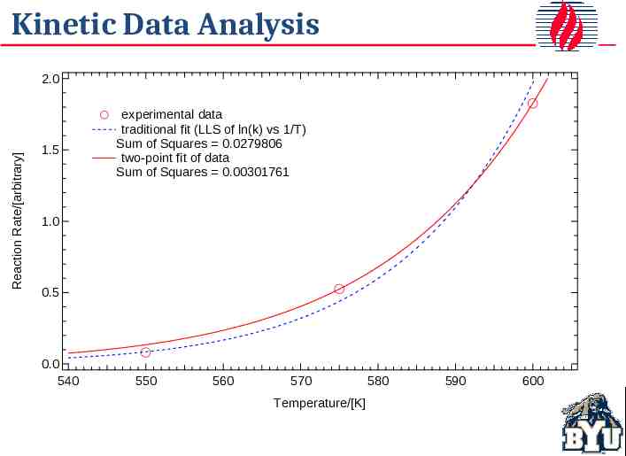
Kinetic Data Analysis Reaction Rate/[arbitrary] 2.0 1.5 experimental data traditional fit (LLS of ln(k) vs 1/T) Sum of Squares 0.0279806 two-point fit of data Sum of Squares 0.00301761 1.0 0.5 0.0 540 550 560 570 Temperature/[K] 580 590 600

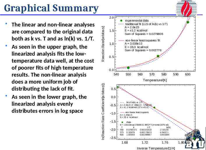
Graphical Summary 1.5 1.0 experimental data traditional fit (LLS of ln(k) vs 1/T) A 2.0e15 E 41.2 kcal/mol Sum of Squares 0.0279806 non-linear least-squares fit A 3.038e13 E 36.3 kcal/mol Sum of Squares 0.002776 0.5 0.0 540 550 560 570 580 590 600 Temperature/[K] ln(Reaction Rate Coefficient/[arbitrary]) The linear and non-linear analyses are compared to the original data both as k vs. T and as ln(k) vs. 1/T. As seen in the upper graph, the linearized analysis fits the lowtemperature data well, at the cost of poorer fits of high temperature results. The non-linear analysis does a more uniform job of distributing the lack of fit. As seen in the lower graph, the linearized analysis evenly distributes errors in log space Reaction Rate/[arbitrary] 2.0 0.5 0.0 -0.5 -1.0 -1.5 -2.0 fit of ln(k) vs 1/T A 2.0e15 (7.166e13 - 5.59e16) E 41.2 kcal/mol (37.4-45.0) non-linear least squares A 1.45e13 E 35.4 kcal/mol data k 1.0e13exp(-35000/(1.9872*T)) noise(10% sd) T k 1/T ln(k) 550 0.0795571 0.00181818 -2.53128 575 0.52429 0.00173913 -0.64571 600 1.82548 0.00166667 0.601844 -2.5 1.68 1.72 1.76 Inverse Temperature/[1/K] -3 1.80x10

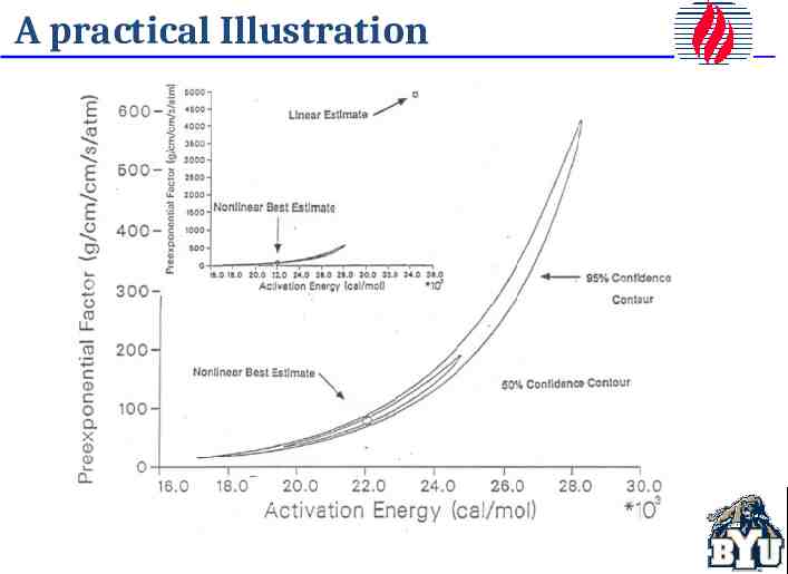
A practical Illustration

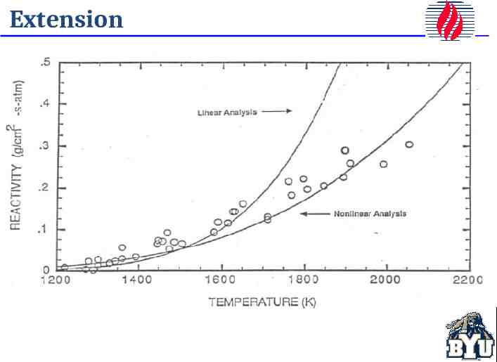
Extension

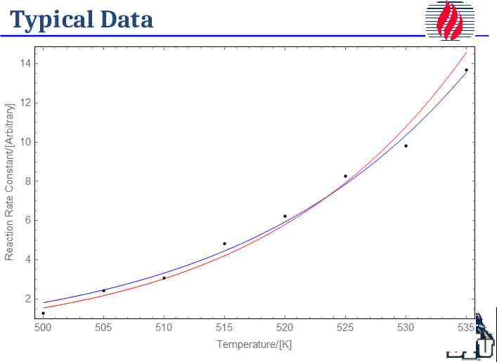
Typical Data

Parameter Estimates Best estimate of parameters for a given set of data. Linear Equations Explicit equations Requires no initial guess Depends only on measured values of dependent and independent variables Does not depend on values of any other parameters Nonlinear Equations Implicit equations Requires initial guess Convergence often difficult Depends on data and on parameters

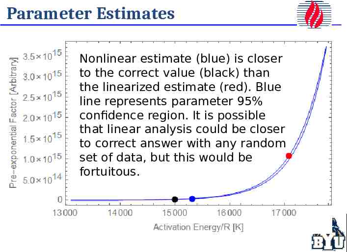
Parameter Estimates Nonlinear estimate (blue) is closer to the correct value (black) than the linearized estimate (red). Blue line represents parameter 95% confidence region. It is possible that linear analysis could be closer to correct answer with any random set of data, but this would be fortuitous.

For Parameter Estimates In all cases, linear and nonlinear, fit what you measure, or more specifically the data that have normally distributed errors, rather than some transformation of this. Any nonlinear transformation (something other than adding or multiplying by a constant) changes the error distribution and invalidates much of the statistical theory behind the analysis. Standard packages are widely available for linear equations. Nonlinear analyses should be done on raw data (or data with normally distributed errors) and will require iteration, which Excel and other programs can handle.

Experimental Error The inherent error in the data figures prominently into almost all analyses except the best estimates of the parameters. The classical assumptions are that these errors are additive, normally distributed with a mean of 0 and constant variance (independent of the value of the dependent and independent variables and of time), and independent. None of these assumptions is always true. Errors could be multiplicative with mean of 1, but this is equivalent to additive with mean 0 but proportional to the predicted value. Could have other forms. Errors may be non-normally distributed, but the Central Limit Theorem provides reasonably strong motivation for them being normally distributed in many cases. Errors often depend on each other, especially when data come from computerized acquisition systems at high rates.

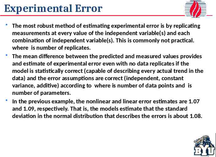
Experimental Error The most robust method of estimating experimental error is by replicating measurements at every value of the independent variable(s) and each combination of independent variable(s). This is commonly not practical. where is number of replicates. The mean difference between the predicted and measured values provides and estimate of experimental error even with no data replicates if the model is statistically correct (capable of describing every actual trend in the data) and the error assumptions are correct (independent, constant variance, additive) according to where is number of data points and is number of parameters. In the previous example, the nonlinear and linear error estimates are 1.07 and 1.09, respectively. That is, the models estimate that the standard deviation in the normal distribution that describes the errors is about 1.08.

Population vs Sample Statistics There are two common definitions of a standard deviation that sometimes lead to confusion. is the sample estimate. That is, it is the estimated standard deviation based on a sample set of data drawn from a usually much larger population when the mean is also based on this sample set of data. Excel functions STDEV() and STDEV.S() return this value for a list of data. is the population estimate. That is, it is the standard deviation based on the entire population or based on a sample when the mean is known or estimated from some independent source. Excel functions STDEVP() and STDEV.P() return this value for a list of data.

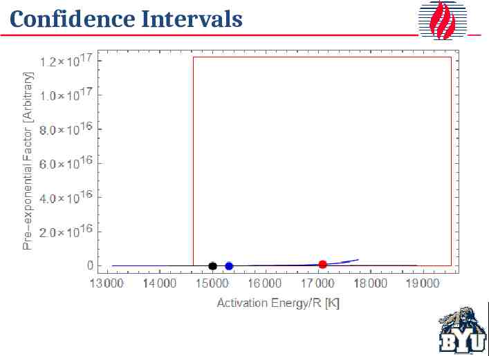
Confidence Intervals

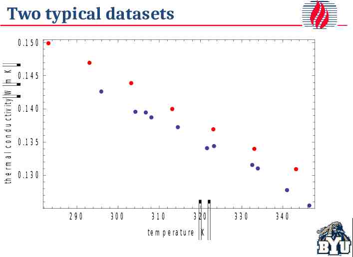
Two typical datasets th e r m a l c o n d u c tiv ity W m K 0 .1 5 0 0 .1 4 5 0 .1 4 0 0 .1 3 5 0 .1 3 0 290 300 310 320 te m p e ra tu re K 330 340

Straight-line Regression 0 .1 5 0 th e r m a l c o n d u c tiv ity W m K Estimate Std Error t-Statistic P-Value intercept 0.241001 1.733e-4 139.041 3.6504e-10 slope -3.214e-4 5.525e-6 -58.1739 2.8398e-8 0 .1 4 5 0 .1 4 0 0 .1 3 5 0 .1 3 0 Estimate Std Error t-Statistic P-Value intercept 0.239396 3.3021e-372.4977 9.13934e-14 slope -3.264e-4 1.0284e-5-31.7349 1.50394e-10 290 300 310 320 te m p e ra tu re K 330 340

Mean Prediction Bands

Single-Point Prediction Bands

Point and Mean Prediction Bands

Rigorous vs. Propagation of Error NaCl Liquid Thermal Conductivity - W/m K 1.03 Data Best Fit 95% CI for Best Fit -95% CI for Best Fit 95% CI using PD -95% CI using PD 1.02 Ratio PD:rigorous CI at avg x 49 1.01 1 1080 1100 1120 1140 1160 Temperature - K 1180 1200 1220

Propagation of Error

Single-Point Prediction Band

Residual SP Prediction Band (95%)

Confidence Region linearized result correct (unknown) result nonlinear result

Joint Confidence Regions linearized result nonlinear result

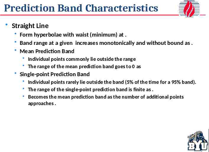
Prediction Band Characteristics Straight Line Form hyperbolae with waist (minimum) at . Band range at a given increases monotonically and without bound as . Mean Prediction Band Individual points commonly lie outside the range The range of the mean prediction band goes to 0 as Single-point Prediction Band Individual points rarely lie outside the band (5% of the time for a 95% band). The range of the single-point prediction band is finite as . Becomes the mean prediction band as the number of additional points approaches .

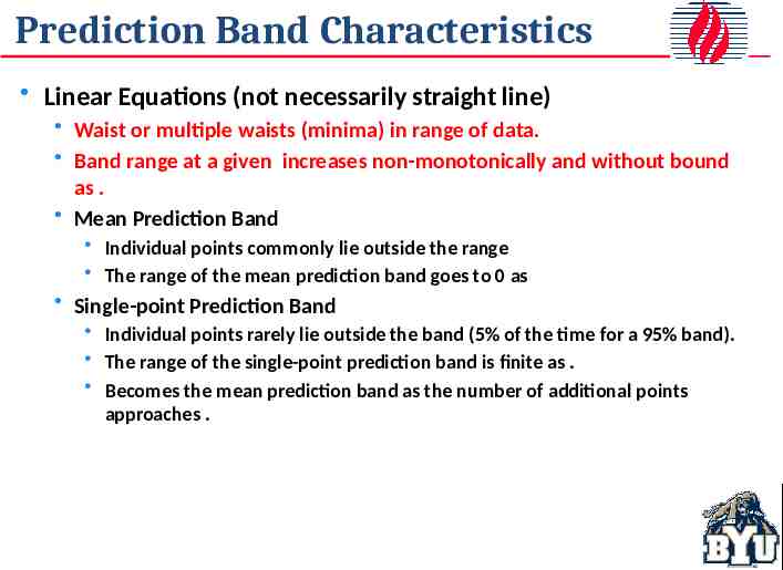
Prediction Band Characteristics Linear Equations (not necessarily straight line) Waist or multiple waists (minima) in range of data. Band range at a given increases non-monotonically and without bound as . Mean Prediction Band Individual points commonly lie outside the range The range of the mean prediction band goes to 0 as Single-point Prediction Band Individual points rarely lie outside the band (5% of the time for a 95% band). The range of the single-point prediction band is finite as . Becomes the mean prediction band as the number of additional points approaches .

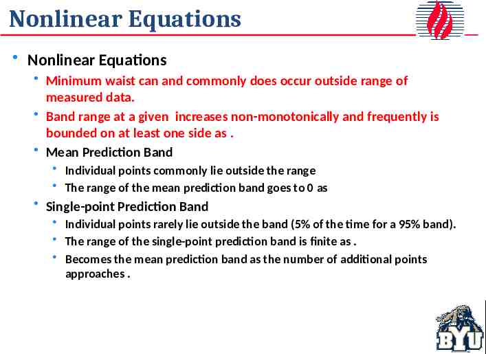
Nonlinear Equations Nonlinear Equations Minimum waist can and commonly does occur outside range of measured data. Band range at a given increases non-monotonically and frequently is bounded on at least one side as . Mean Prediction Band Individual points commonly lie outside the range The range of the mean prediction band goes to 0 as Single-point Prediction Band Individual points rarely lie outside the band (5% of the time for a 95% band). The range of the single-point prediction band is finite as . Becomes the mean prediction band as the number of additional points approaches .

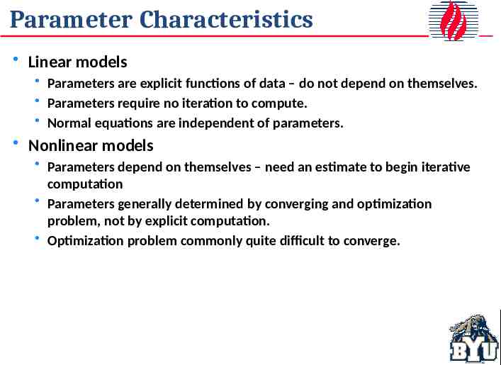
Parameter Characteristics Linear models Parameters are explicit functions of data – do not depend on themselves. Parameters require no iteration to compute. Normal equations are independent of parameters. Nonlinear models Parameters depend on themselves – need an estimate to begin iterative computation Parameters generally determined by converging and optimization problem, not by explicit computation. Optimization problem commonly quite difficult to converge.

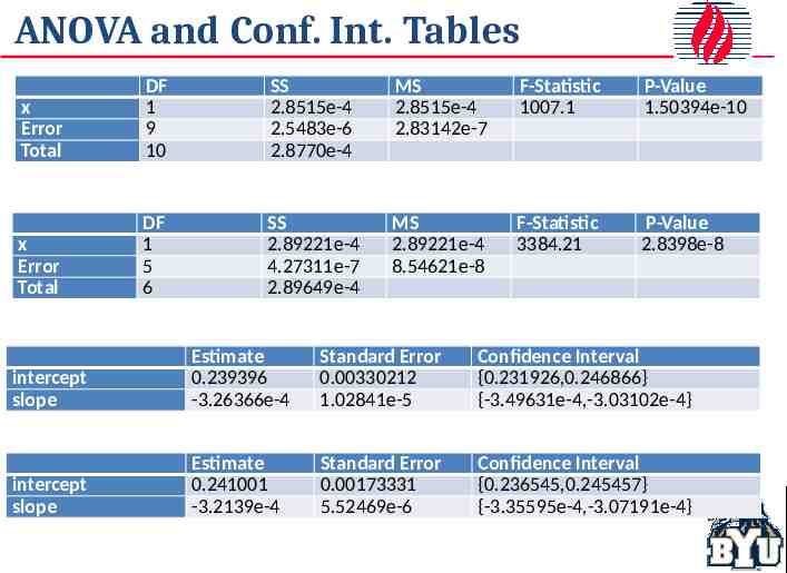
ANOVA and Conf. Int. Tables x Error Total DF 1 9 10 SS 2.8515e-4 2.5483e-6 2.8770e-4 MS 2.8515e-4 2.83142e-7 F-Statistic 1007.1 P-Value 1.50394e-10 x Error Total DF 1 5 6 SS 2.89221e-4 4.27311e-7 2.89649e-4 MS 2.89221e-4 8.54621e-8 F-Statistic 3384.21 P-Value 2.8398e-8 intercept slope Estimate 0.239396 -3.26366e-4 Standard Error 0.00330212 1.02841e-5 Confidence Interval {0.231926,0.246866} {-3.49631e-4,-3.03102e-4} intercept slope Estimate 0.241001 -3.2139e-4 Standard Error 0.00173331 5.52469e-6 Confidence Interval {0.236545,0.245457} {-3.35595e-4,-3.07191e-4}

Confidence Interval Ranges

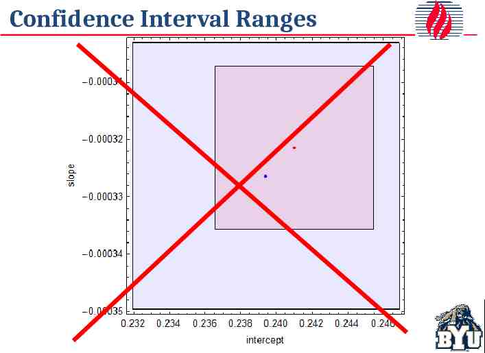
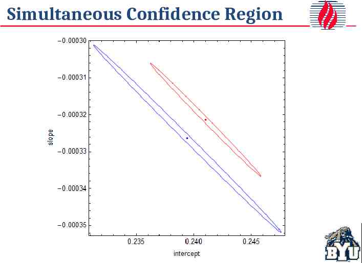
Some Interpretation Traps It would be easy, but incorrect, to conclude That reasonable estimates of the line can, within 95% probability, be computed by any combination of parameters within the 95% confidence interval for each parameter That experiments that overlap represent the same experimental results, within 95% confidence That parameters with completely overlapped confidence intervals represent essentially indistinguishable results If you consider the first graph in this case, all of these conclusions seem intuitively incorrect, but experimenters commonly draw these types of conclusions. Joint or simultaneous confidence regions (SCR) address these problems

Simultaneous Confidence Region

Regions and Intervals Compared

Nonlinear SCR More Complex The Cauchy or Nonlinear parameter simultaneous confidence region(s) are defined Lorentz in general by the equation equation (is a probability density function and describes some laser line widths).1 𝑦 ( 𝑥 𝑎)2 1 2 𝑏 In this case, there are 4 noncontiguous regions.

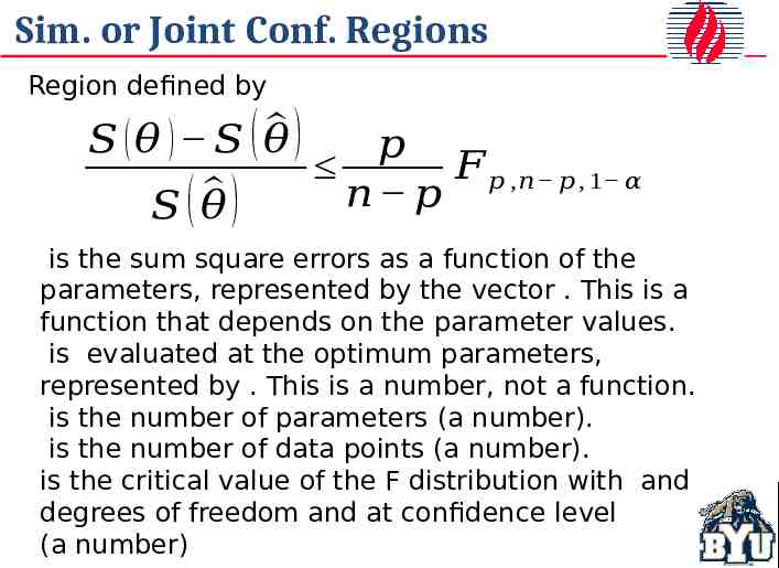
Sim. or Joint Conf. Regions Region defined by ) 𝑆 (𝜃 ) 𝑆 ( 𝜃 𝑝 𝐹 𝑝 ,𝑛 𝑝 , 1 𝛼 ) 𝑛 𝑝 𝑆(𝜃 is the sum square errors as a function of the parameters, represented by the vector . This is a function that depends on the parameter values. is evaluated at the optimum parameters, represented by . This is a number, not a function. is the number of parameters (a number). is the number of data points (a number). is the critical value of the F distribution with and degrees of freedom and at confidence level (a number)

Simultaneous Confidence Regions Overlapping confidence intervals is a poor test for difference in data sets. Data that may appear to be similar based on confidence intervals may in fact be quite different and certainly distinct from one another. Parameters in the lonely corners of interval unions are exceptionally poor estimates.

Confidence Region Characteristics Linear Equations Always form -dimensional ellipsoids, where is the number of parameters. Parameters are generally linearly correlated (ellipsoid axes are not aligned with parameter axes). Not correlated for straight line if . Constant and quadratic parameters always correlated for quadratic Parameter uncertainty is usually much smaller than confidence interval at given values of other parameters. Parameter uncertainty range slightly exceeds conf. interval range.

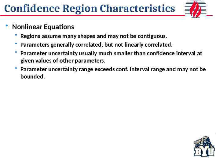
Confidence Region Characteristics Nonlinear Equations Regions assume many shapes and may not be contiguous. Parameters generally correlated, but not linearly correlated. Parameter uncertainty usually much smaller than confidence interval at given values of other parameters. Parameter uncertainty range exceeds conf. interval range and may not be bounded.

Experimental Design In this context, experimental design means selecting the conditions that will maximize the accuracy of your model for a fixed number of experiments. There are many experimental designs, depending on whether you want to maximize accuracy of prediction band, all parameters simultaneously, a subset of the parameters, etc. The d-optimal design maximizes the accuracy of all parameters and is quite close to best designs for other criteria. It is, therefore, by far the most widely used.

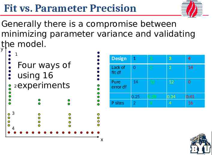
Fit vs. Parameter Precision Generally there is a compromise between minimizing parameter variance and validating the model. y 1 Four ways of using 16 2 experiments Design 1 2 3 4 Lack of fit df 0 2 2 14 Pure error df 14 12 12 0 0.25 2 0.28 4 0.34 4 0.41 16 P sites 3 4 x

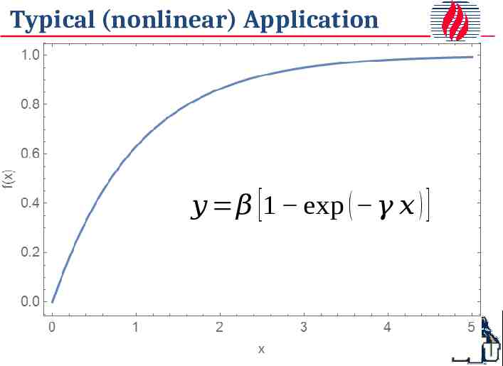
Typical (nonlinear) Application 𝑦 𝛽 [ 1 exp ( 𝛾 𝑥 ) ]

Example Compare 3 different design, each with the same number of data points and the same errors Point No. 1 2 3 4 5 6 7 8 9 10 0.1 0.2 0.3 0.4 0.5 0.6 0.7 0.8 0.9 1.0 0.0638 0.1870 0.2495 0.3207 0.3356 0.5040 0.5030 0.6421 0.6412 0.5678 0.1 0.6 1.1 1.6 2.1 2.6 3.1 3.6 4.1 4.6 0.0638 0.4569 0.6574 0.7891 0.8197 0.9786 0.9545 1.0461 1.0312 0.9256 0.954 0.954 0.954 0.954 0.954 4.605 4.605 4.605 4.605 4.605 0.5833 0.6203 0.6049 0.6056 0.5567 1.0428 0.9896 1.0634 1.0377 0.9257 0.03150 -0.00550 0.00990 0.00920 0.05810 -0.05280 0.00040 -0.07340 -0.04770 0.06430

SCR Results for 3 Cases 10 points equally spaced where Y changes fastest (0-1) 10 equally spaced points between 0 and 4.6 Optimal design (5 pts at 0.95 and 5 pts at 4.6)

Prediction and SP Conf. Intervals Optimal design (blue) improves predictions everywhere. Recall data for optimal design regression were all at two points, 0.95 and 4.6.

Improved Prediction & SP Intervals Optimal design (blue) improves predictions everywhere, including extrapolated regions. Recall data for optimal design regression were all at two points, 0.95 and 4.6.

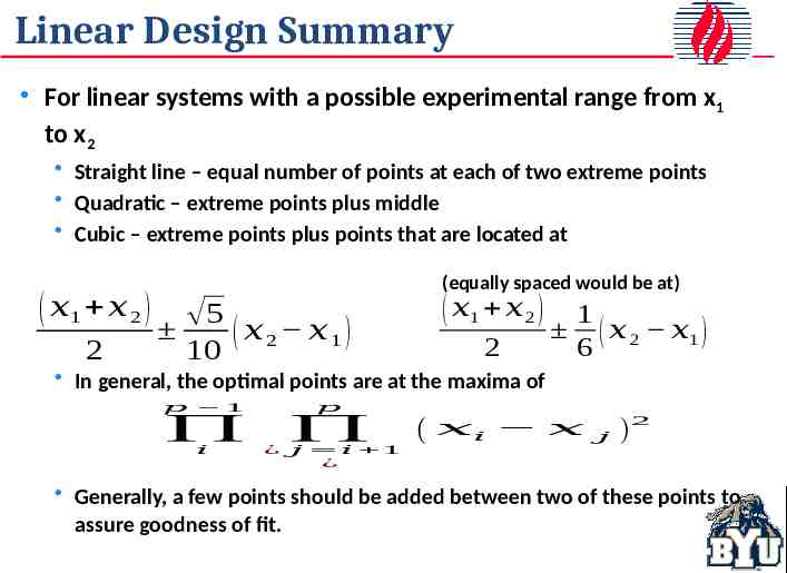
Linear Design Summary For linear systems with a possible experimental range from x1 to x2 Straight line – equal number of points at each of two extreme points Quadratic – extreme points plus middle Cubic – extreme points plus points that are located at ( 𝑥1 𝑥 2 ) 2 (equally spaced would be at) 5 𝑥2 𝑥1) ( 10 ( 𝑥1 𝑥 2 ) 2 1 ( 𝑥 2 𝑥1 ) 6 In general, the optimal points are at the maxima of 𝑝 1 𝑝 𝑖 ¿ 𝑗 𝑖 1 ¿ ( 𝑥𝑖 𝑥 𝑗 ) 2 Generally, a few points should be added between two of these points to assure goodness of fit.

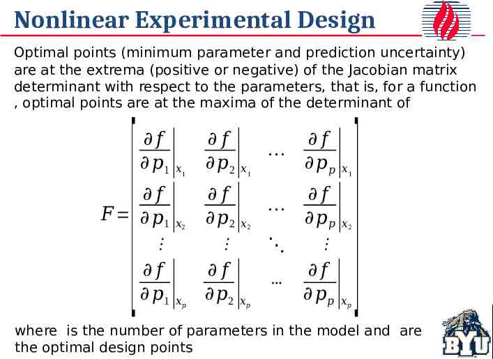
Nonlinear Experimental Design Optimal points (minimum parameter and prediction uncertainty) are at the extrema (positive or negative) of the Jacobian matrix determinant with respect to the parameters, that is, for a function , optimal points are at the maxima of the determinant of [ 𝑓 𝑝1 𝑓 𝐹 𝑝1 𝑓 𝑝1 𝑥1 𝑥2 𝑥𝑝 𝑓 𝑝2 𝑥1 𝑓 𝑝2 𝑥 𝑓 𝑝2 𝑥 2 𝑝 𝑓 𝑝𝑝 2 𝑝 𝑥1 𝑓 𝑝𝑝 𝑥 𝑓 𝑝𝑝 𝑥 ] where is the number of parameters in the model and are the optimal design points

Nonlinear Design Summary Nonlinear design depends on the value of parameters. Determining the parameters is usually the objective of the design. A bit of a circular (iterative) process. Start with reasonable estimates. The design can be stated as finding the maxima of or the extrema of . The latter is simpler math. In many but not all cases, one or more extrema will be at the highest or lowest achievable value of the independent variable. There will be at least inflection points, located at . These are optimally poor (useless), not optimally good design points. Frequently, the extrema can only be found numerically or graphically, not analytically.

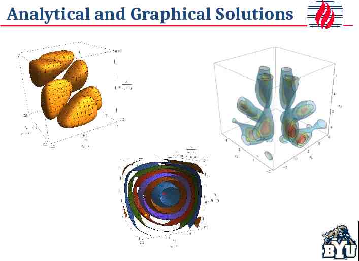
Analytical and Graphical Solutions

Conclusions Statistics is the primary means of inductive logic in the technical world. With proper statistics, we can move from specific results to general statements with known accuracy ranges in the general statements. Many aspects of linear statistics are commonly misunderstood or misinterpreted. Nonlinear statistics is a generalization of linear statistics (becomes identical as the model becomes more linear) but most of the results and the math are more complex. Statistics is highly useful in both designing and analyzing experiments.