LOGISTICS PLANNING Dr M MATHIRAJAN Department of Management

45 Slides576.00 KB
LOGISTICS PLANNING Dr M MATHIRAJAN Department of Management Studies Indian Institute of Science Bangalore
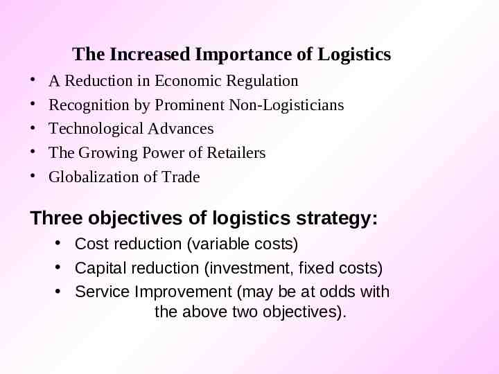
The Increased Importance of Logistics A Reduction in Economic Regulation Recognition by Prominent Non-Logisticians Technological Advances The Growing Power of Retailers Globalization of Trade Three objectives of logistics strategy: Cost reduction (variable costs) Capital reduction (investment, fixed costs) Service Improvement (may be at odds with the above two objectives).
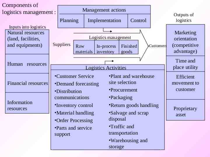
Components of logistics management : Management actions Planning Implementation Outputs of logistics Control Inputs into logistics Natural resources (land, facilities, and equipments) Human resources Financial resources Information resources Logistics management Suppliers Raw In-process materials inventory Finished goods Customers Logistics Activities Customer Service Demand forecasting Distribution communications Inventory control Material handling Order Processing Parts and service support Plant and warehouse site selection Procurement Packaging Return goods handling Salvage and scrap disposal Traffic and transportation Warehousing and storage Marketing orientation (competitive advantage) Time and place utility Efficient movement to customer Proprietary asset
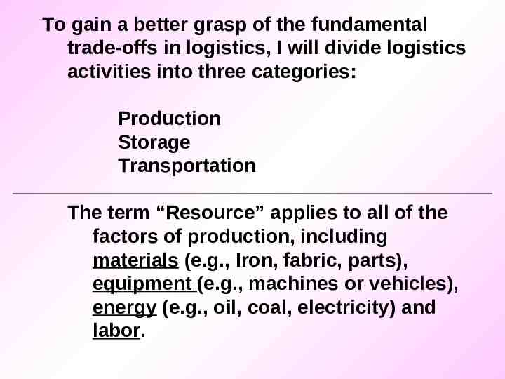
To gain a better grasp of the fundamental trade-offs in logistics, I will divide logistics activities into three categories: Production Storage Transportation The term “Resource” applies to all of the factors of production, including materials (e.g., Iron, fabric, parts), equipment (e.g., machines or vehicles), energy (e.g., oil, coal, electricity) and labor.
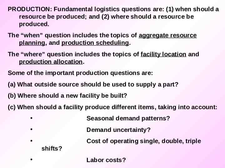
PRODUCTION: Fundamental logistics questions are: (1) when should a resource be produced; and (2) where should a resource be produced. The “when” question includes the topics of aggregate resource planning, and production scheduling. The “where” question includes the topics of facility location and production allocation. Some of the important production questions are: (a) What outside source should be used to supply a part? (b) Where should a new facility be built? (c) When should a facility produce different items, taking into account: Seasonal demand patterns? Demand uncertainty? Cost of operating single, double, triple shifts? Labor costs?
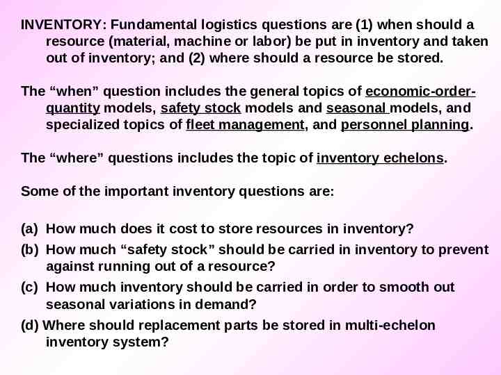
INVENTORY: Fundamental logistics questions are (1) when should a resource (material, machine or labor) be put in inventory and taken out of inventory; and (2) where should a resource be stored. The “when” question includes the general topics of economic-orderquantity models, safety stock models and seasonal models, and specialized topics of fleet management, and personnel planning. The “where” questions includes the topic of inventory echelons. Some of the important inventory questions are: (a) How much does it cost to store resources in inventory? (b) How much “safety stock” should be carried in inventory to prevent against running out of a resource? (c) How much inventory should be carried in order to smooth out seasonal variations in demand? (d) Where should replacement parts be stored in multi-echelon inventory system?
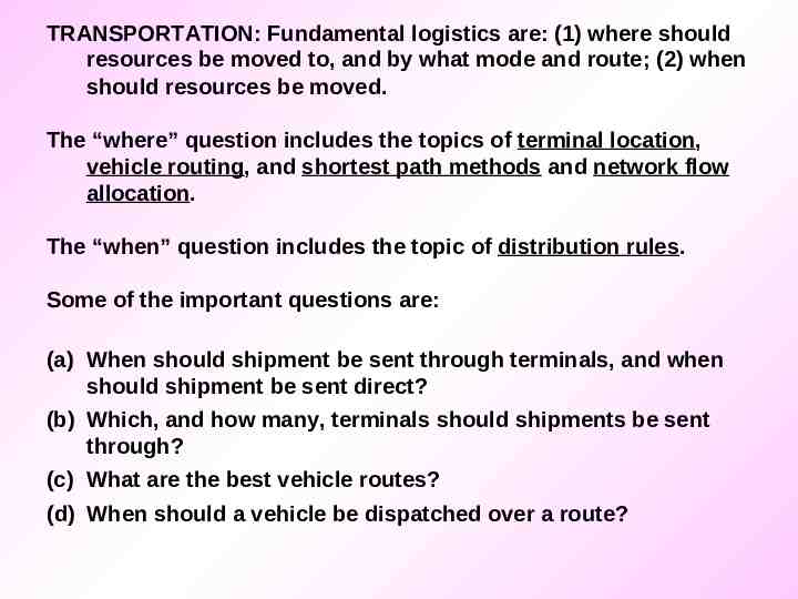
TRANSPORTATION: Fundamental logistics are: (1) where should resources be moved to, and by what mode and route; (2) when should resources be moved. The “where” question includes the topics of terminal location, vehicle routing, and shortest path methods and network flow allocation. The “when” question includes the topic of distribution rules. Some of the important questions are: (a) When should shipment be sent through terminals, and when should shipment be sent direct? (b) Which, and how many, terminals should shipments be sent through? (c) What are the best vehicle routes? (d) When should a vehicle be dispatched over a route?
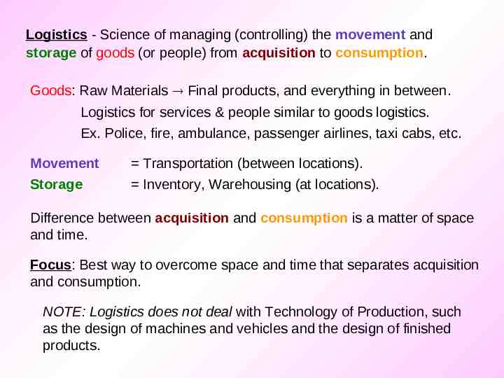
Logistics - Science of managing (controlling) the movement and storage of goods (or people) from acquisition to consumption. Goods: Raw Materials Final products, and everything in between. Logistics for services & people similar to goods logistics. Ex. Police, fire, ambulance, passenger airlines, taxi cabs, etc. Movement Transportation (between locations). Storage Inventory, Warehousing (at locations). Difference between acquisition and consumption is a matter of space and time. Focus: Best way to overcome space and time that separates acquisition and consumption. NOTE: Logistics does not deal with Technology of Production, such as the design of machines and vehicles and the design of finished products.
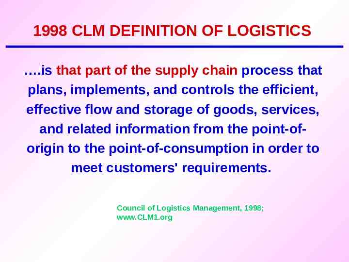
1998 CLM DEFINITION OF LOGISTICS .is that part of the supply chain process that plans, implements, and controls the efficient, effective flow and storage of goods, services, and related information from the point-oforigin to the point-of-consumption in order to meet customers' requirements. Council of Logistics Management, 1998; www.CLM1.org
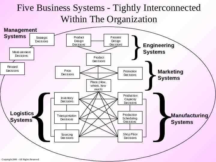
Five Business Systems - Tightly Interconnected Within The Organization Management Systems Strategic Decisions Product Design Decisions Measurement Decisions Reward Decisions Process Design Decisions Product Decisions Price Decisions { Logistics Systems Copyright 2000 - All Rights Reserved } Engineering Systems Promotion Decisions Place (How, where, how much) Inventory Decisions Production Capacity Decisions Transportation Decisions Production Scheduling Decisions Sourcing Decisions Shop Floor Decisions } Marketing Systems } Manufacturing Systems
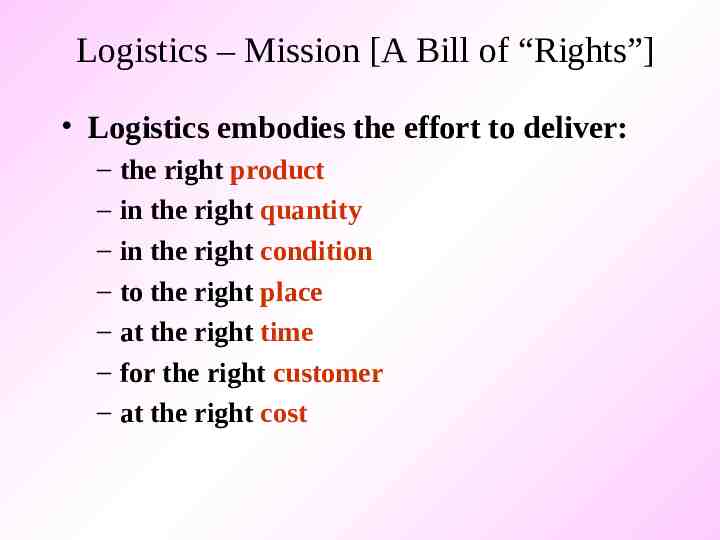
Logistics – Mission [A Bill of “Rights”] Logistics embodies the effort to deliver: – – – – – – – the right product in the right quantity in the right condition to the right place at the right time for the right customer at the right cost
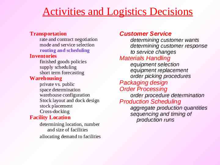
Activities and Logistics Decisions Transportation rate and contract negotiation mode and service selection routing and scheduling Inventories finished goods policies supply scheduling short term forecasting Warehousing private vs. public space determination warehouse configuration Stock layout and dock design stock placement Cross-docking Facility Location determining location, number and size of facilities allocating demand to facilities Customer Service determining customer wants determining customer response to service changes Materials Handling equipment selection equipment replacement order picking procedures Packaging design Order Processing order procedure determination Production Scheduling aggregate production quantities sequencing and timing of production runs
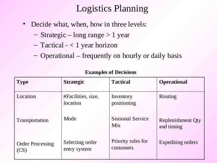
Logistics Planning Decide what, when, how in three levels: – Strategic – long range 1 year – Tactical - 1 year horizon – Operational – frequently on hourly or daily basis Examples of Decisions Type Strategic Tactical Operational Location #Facilities, size, location Inventory positioning Routing Transportation Mode Seasonal Service Mix Replenishment Qty and timing Order Processing (CS) Selecting order entry system Priority rules for customers Expediting orders
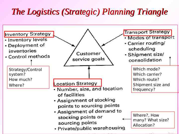
The Logistics (Strategic) Planning Triangle Strategy/Control system? How much? Where? Which mode? Which carrier? Which route? Shipment size and frequency? Where?, How many? What size? Allocation?
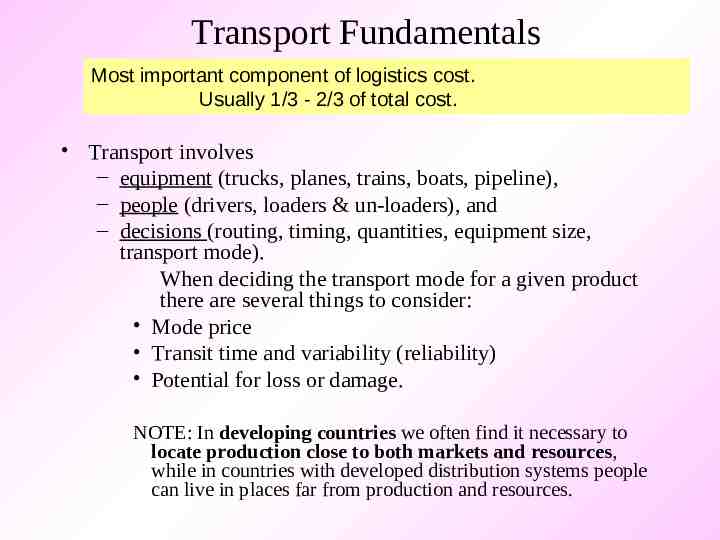
Transport Fundamentals Most important component of logistics cost. Usually 1/3 - 2/3 of total cost. Transport involves – equipment (trucks, planes, trains, boats, pipeline), – people (drivers, loaders & un-loaders), and – decisions (routing, timing, quantities, equipment size, transport mode). When deciding the transport mode for a given product there are several things to consider: Mode price Transit time and variability (reliability) Potential for loss or damage. NOTE: In developing countries we often find it necessary to locate production close to both markets and resources, while in countries with developed distribution systems people can live in places far from production and resources.
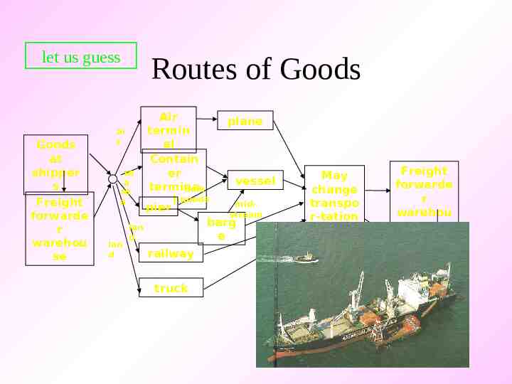
let us guess Goods at shipper s Freight forwarde r warehou se Routes of Goods Air plane termin ai r al Contain se er vessel a termina bulk se l goods a midpier stream barg lan e d lan d railway truck May change transpo r-tation modes Freight forwarde r warehou se Goods at consigne es
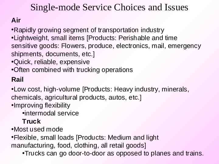
Single-mode Service Choices and Issues Air Rapidly growing segment of transportation industry Lightweight, small items [Products: Perishable and time sensitive goods: Flowers, produce, electronics, mail, emergency shipments, documents, etc.] Quick, reliable, expensive Often combined with trucking operations Rail Low cost, high-volume [Products: Heavy industry, minerals, chemicals, agricultural products, autos, etc.] Improving flexibility intermodal service Truck Most used mode Flexible, small loads [Products: Medium and light manufacturing, food, clothing, all retail goods] Trucks can go door-to-door as opposed to planes and trains.
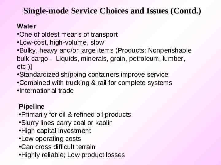
Single-mode Service Choices and Issues (Contd.) Water One of oldest means of transport Low-cost, high-volume, slow Bulky, heavy and/or large items (Products: Nonperishable bulk cargo - Liquids, minerals, grain, petroleum, lumber, etc )] Standardized shipping containers improve service Combined with trucking & rail for complete systems International trade Pipeline Primarily for oil & refined oil products Slurry lines carry coal or kaolin High capital investment Low operating costs Can cross difficult terrain Highly reliable; Low product losses
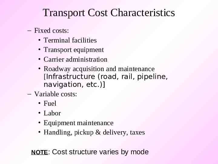
Transport Cost Characteristics – Fixed costs: Terminal facilities Transport equipment Carrier administration Roadway acquisition and maintenance [Infrastructure (road, rail, pipeline, navigation, etc.)] – Variable costs: Fuel Labor Equipment maintenance Handling, pickup & delivery, taxes NOTE: Cost structure varies by mode
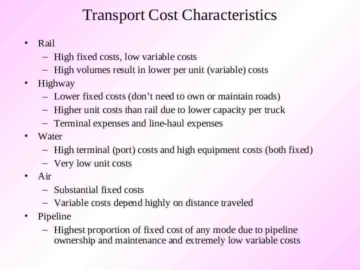
Transport Cost Characteristics Rail – High fixed costs, low variable costs – High volumes result in lower per unit (variable) costs Highway – Lower fixed costs (don’t need to own or maintain roads) – Higher unit costs than rail due to lower capacity per truck – Terminal expenses and line-haul expenses Water – High terminal (port) costs and high equipment costs (both fixed) – Very low unit costs Air – Substantial fixed costs – Variable costs depend highly on distance traveled Pipeline – Highest proportion of fixed cost of any mode due to pipeline ownership and maintenance and extremely low variable costs
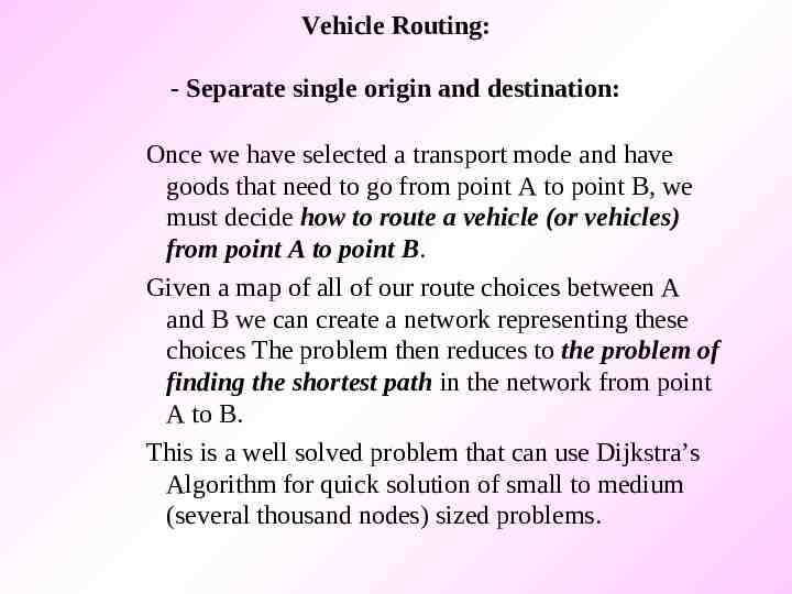
Vehicle Routing: - Separate single origin and destination: Once we have selected a transport mode and have goods that need to go from point A to point B, we must decide how to route a vehicle (or vehicles) from point A to point B. Given a map of all of our route choices between A and B we can create a network representing these choices The problem then reduces to the problem of finding the shortest path in the network from point A to B. This is a well solved problem that can use Dijkstra’s Algorithm for quick solution of small to medium (several thousand nodes) sized problems.
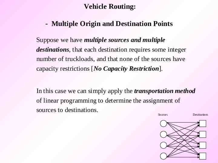
Vehicle Routing: - Multiple Origin and Destination Points Suppose we have multiple sources and multiple destinations, that each destination requires some integer number of truckloads, and that none of the sources have capacity restrictions [No Capacity Restriction]. In this case we can simply apply the transportation method of linear programming to determine the assignment of sources to destinations. Sources Destinations
Vehicle Routing: - Coincident Origin and Destination: The TSP If a vehicle must deliver to more than two customers, we must decide the order in which we will visit those customers so as to minimize the total cost of making the delivery. We first suppose that any time that we make a delivery to customers we are able to make use of only a single vehicle, i.e., that vehicle capacity of our only truck is never an issue. In this case, we need to dispatch a single vehicle from our depot to n - 1 customers, with the vehicle returning to the depot following its final delivery. This is the well-known Traveling Salesman Problem (TSP). The TSP has been well studied and solved for problem instances involving thousands of nodes. We can formulate the TSP as follows:
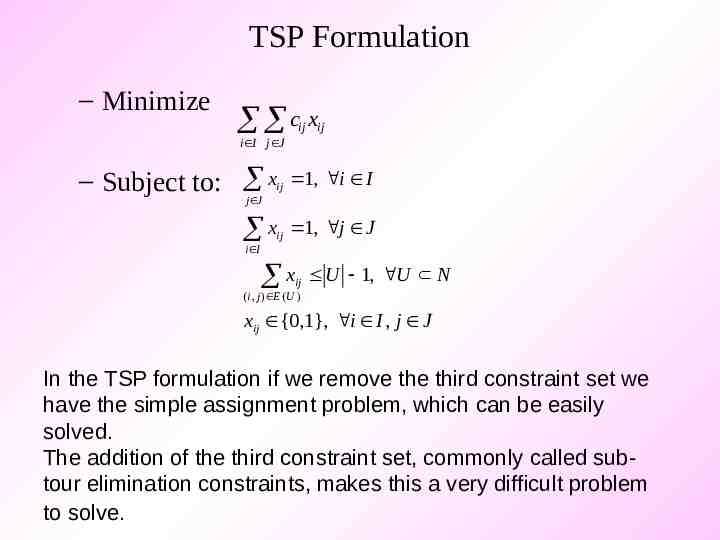
TSP Formulation – Minimize c x ij ij i I j J – Subject to: xij 1, i I j J x ij 1, j J i I x ij ( i , j ) E (U ) U 1, U N xij {0,1}, i I , j J In the TSP formulation if we remove the third constraint set we have the simple assignment problem, which can be easily solved. The addition of the third constraint set, commonly called subtour elimination constraints, makes this a very difficult problem to solve.
Questions about the TSP Given a problem with n nodes, how many distinct feasible tours exist? How many arcs will the network have? How many xij variables will we have? How could we quantify the number of subtour elimination constraints? The complexity of the TSP has led to several heuristic or approximate methods for finding good feasible solutions. The simplest solution we might think of is that of the nearest neighbor.
Vehicle Routing: TSP, inventory routing, and vehicle routing Traveling Salesman Problem (TSP): salesman visits n cities at minimum cost vehicle routing problem (VRP): m vehicles with capacity to deliver to n customers who have volume requirement, time windows, etc. Inventory Routing: m vehicle to delivery to n customer with time windows, vehicle and storage capacity constraints, and unspecificed amount to be delivered. Heuristics 1. Load points closest together on the same truck 2. Build routes starting with points farther from depot first 3. Fill the largest vehicle to capacity first 4. Routes should not cross 5. Form teardrop pattern routes. 6. Plan pickups during deliveries, not after all deliveries have been made.
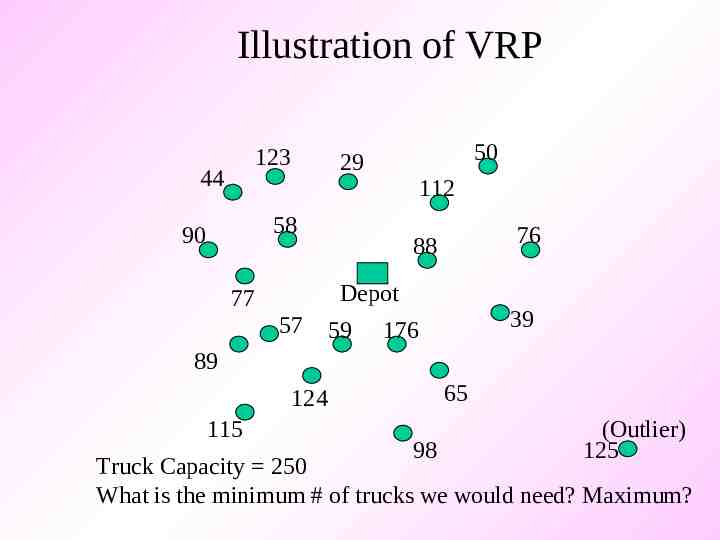
Illustration of VRP 123 44 50 29 112 58 90 77 76 88 Depot 57 59 39 176 89 65 124 115 98 (Outlier) 125 Truck Capacity 250 What is the minimum # of trucks we would need? Maximum?
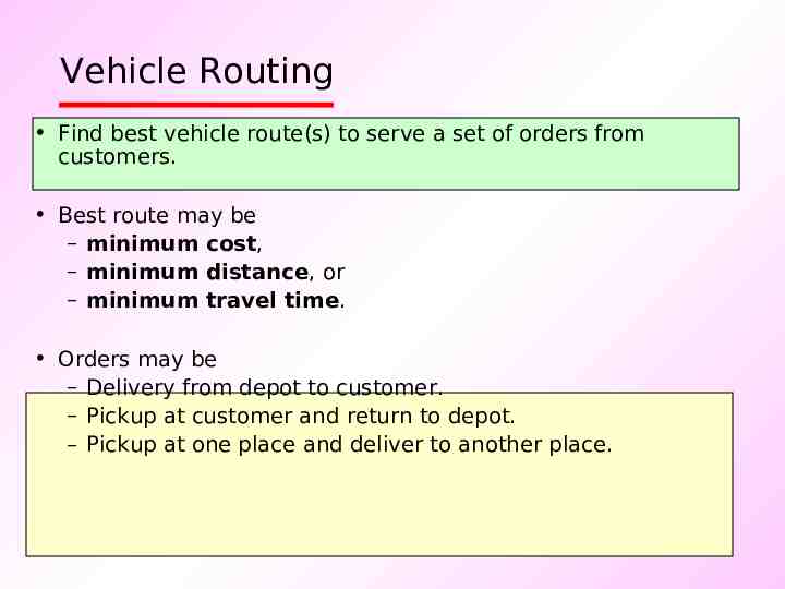
Vehicle Routing Find best vehicle route(s) to serve a set of orders from customers. Best route may be – minimum cost, – minimum distance, or – minimum travel time. Orders may be – Delivery from depot to customer. – Pickup at customer and return to depot. – Pickup at one place and deliver to another place.
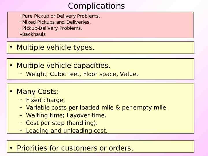
Complications –Pure Pickup or Delivery Problems. –Mixed Pickups and Deliveries. –Pickup-Delivery Problems. –Backhauls Multiple vehicle types. Multiple vehicle capacities. – Weight, Cubic feet, Floor space, Value. Many Costs: – – – – – Fixed charge. Variable costs per loaded mile & per empty mile. Waiting time; Layover time. Cost per stop (handling). Loading and unloading cost. Priorities for customers or orders.
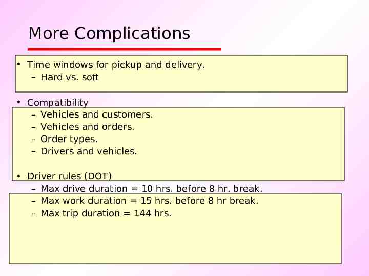
More Complications Time windows for pickup and delivery. – Hard vs. soft Compatibility – Vehicles and customers. – Vehicles and orders. – Order types. – Drivers and vehicles. Driver rules (DOT) – Max drive duration 10 hrs. before 8 hr. break. – Max work duration 15 hrs. before 8 hr break. – Max trip duration 144 hrs.
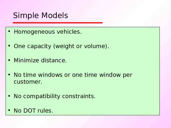
Simple Models Homogeneous vehicles. One capacity (weight or volume). Minimize distance. No time windows or one time window per customer. No compatibility constraints. No DOT rules.
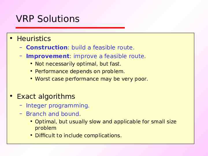
VRP Solutions Heuristics – Construction: build a feasible route. – Improvement: improve a feasible route. Not necessarily optimal, but fast. Performance depends on problem. Worst case performance may be very poor. Exact algorithms – Integer programming. – Branch and bound. Optimal, but usually slow and applicable for small size problem Difficult to include complications.
APPLICATIONS OF VRP The VRP is applicable in many practical situations directly related to the physical delivery of goods such as distribution of petroleum products, distribution of industrial gases, newspaper deliveries, delivery of goods to retail store, garbage collection and disposal, package pick-up and delivery, milk pick-up and delivery, etc. the non-movement of goods such as picking up of students by school buses, routing of salesmen, reading of electric meters, preventive maintenance inspection tours, employee pick-up and drop-off , etc.
COVERS- COMPUTERIZED VEHICLE ROUTING SYSTEM A DSS Employee Bus Routing Commodity Distribution In COVERS Efficient Heuristic Procedures NNH MNNH MSCWH Simulation Features Manipulate the System Generated Routes Completely User Generated Routes COVERS Handles Multi-Depot VRP Heterogeneous VRP
EMPLOYEE PICKUP VEHICLE ROUTING PROBLEM (EPVRP) – BANGALORE, KARNATAKA, INDIA Indian Telephone Industries [ITI] Limited Bharat Electronics Limited [BEL] Hindustan Machine Tools [HMT] Hindustan Aeronautics Limited [HAL] Indian Space Research Organization [ISRO] National Aeronautical Laboratory [NAL] Central Machine Tools of India [CMTI]
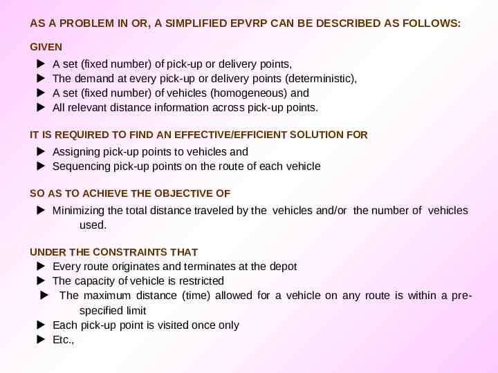
AS A PROBLEM IN OR, A SIMPLIFIED EPVRP CAN BE DESCRIBED AS FOLLOWS: GIVEN A set (fixed number) of pick-up or delivery points, The demand at every pick-up or delivery points (deterministic), A set (fixed number) of vehicles (homogeneous) and All relevant distance information across pick-up points. IT IS REQUIRED TO FIND AN EFFECTIVE/EFFICIENT SOLUTION FOR Assigning pick-up points to vehicles and Sequencing pick-up points on the route of each vehicle SO AS TO ACHIEVE THE OBJECTIVE OF Minimizing the total distance traveled by the vehicles and/or the number of vehicles used. UNDER THE CONSTRAINTS THAT Every route originates and terminates at the depot The capacity of vehicle is restricted The maximum distance (time) allowed for a vehicle on any route is within a prespecified limit Each pick-up point is visited once only Etc.,
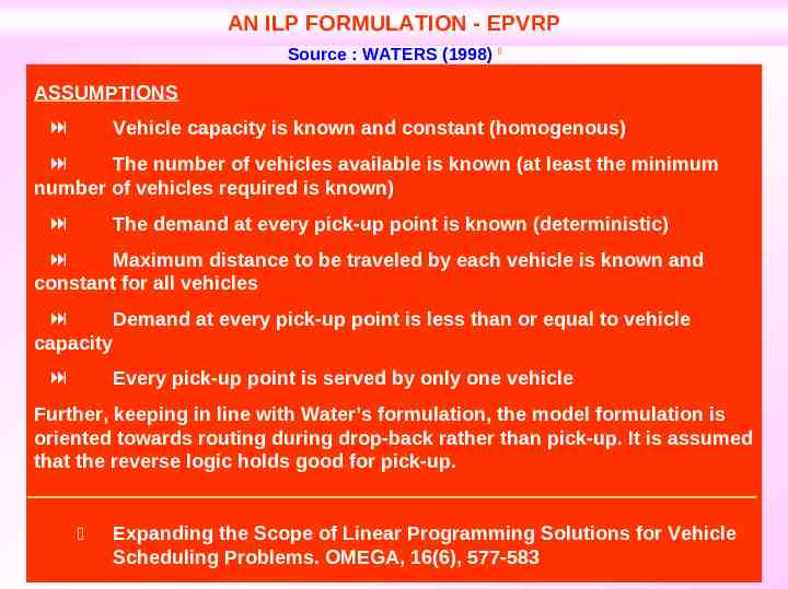
AN ILP FORMULATION - EPVRP Source : WATERS (1998) ASSUMPTIONS Vehicle capacity is known and constant (homogenous) The number of vehicles available is known (at least the minimum number of vehicles required is known) The demand at every pick-up point is known (deterministic) Maximum distance to be traveled by each vehicle is known and constant for all vehicles Demand at every pick-up point is less than or equal to vehicle capacity Every pick-up point is served by only one vehicle Further, keeping in line with Water’s formulation, the model formulation is oriented towards routing during drop-back rather than pick-up. It is assumed that the reverse logic holds good for pick-up. Expanding the Scope of Linear Programming Solutions for Vehicle Scheduling Problems. OMEGA, 16(6), 577-583
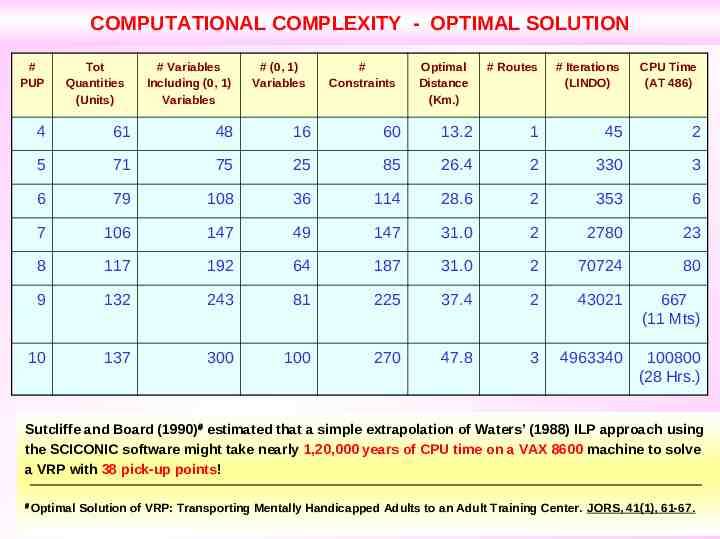
COMPUTATIONAL COMPLEXITY - OPTIMAL SOLUTION # PUP Tot Quantities (Units) # Variables Including (0, 1) Variables # (0, 1) Variables # Constraints Optimal Distance (Km.) # Routes # Iterations (LINDO) CPU Time (AT 486) 4 61 48 16 60 13.2 1 45 2 5 71 75 25 85 26.4 2 330 3 6 79 108 36 114 28.6 2 353 6 7 106 147 49 147 31.0 2 2780 23 8 117 192 64 187 31.0 2 70724 80 9 132 243 81 225 37.4 2 43021 667 (11 Mts) 10 137 300 100 270 47.8 3 4963340 100800 (28 Hrs.) Sutcliffe and Board (1990) estimated that a simple extrapolation of Waters’ (1988) ILP approach using the SCICONIC software might take nearly 1,20,000 years of CPU time on a VAX 8600 machine to solve a VRP with 38 pick-up points! Optimal Solution of VRP: Transporting Mentally Handicapped Adults to an Adult Training Center. JORS, 41(1), 61-67.
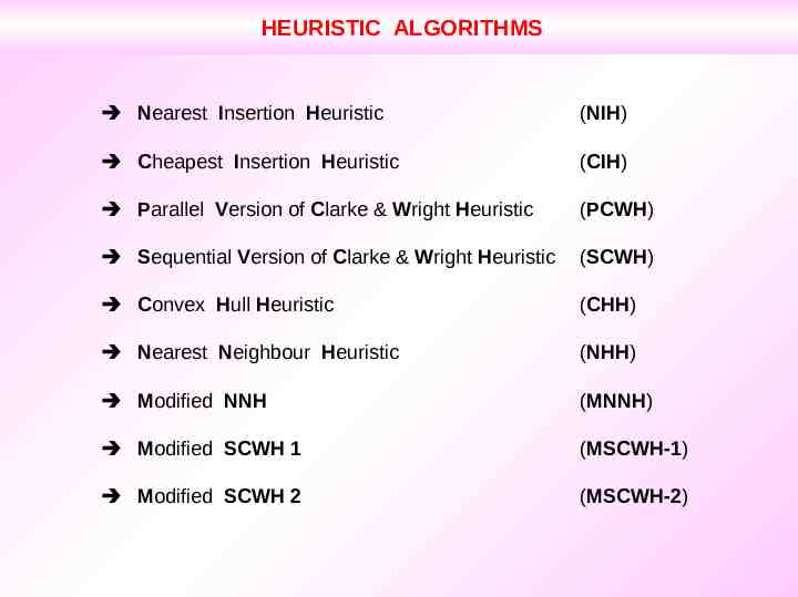
HEURISTIC ALGORITHMS Nearest Insertion Heuristic (NIH) Cheapest Insertion Heuristic (CIH) Parallel Version of Clarke & Wright Heuristic (PCWH) Sequential Version of Clarke & Wright Heuristic (SCWH) Convex Hull Heuristic (CHH) Nearest Neighbour Heuristic (NHH) Modified NNH (MNNH) Modified SCWH 1 (MSCWH-1) Modified SCWH 2 (MSCWH-2)
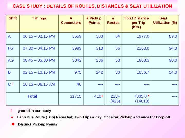
CASE STUDY : DETAILS OF ROUTES, DISTANCES & SEAT UTILIZATION Shift Timings # Commuters # Pickup Points # Routes Total Distance per Trip (Km.) Seat Utilization (%) A 06.15 – 02.15 PM 3659 303 64 1977.0 89.0 FG 07.30 – 04.15 PM 3999 313 66 2163.0 94.3 AG 08.45 – 05.30 PM 3042 286 53 1808.3 90.0 B 02.15 – 10.15 PM 975 242 30 1056.7 54.0 C 10.15 – 06.15 AM 40 ---- ---- ---- ---- 11715 410 213 (426) 7005.0 (14010) ---- Total Ignored in our study Each Bus Route (Trip) Repeated; Two Trips a day, Once for Pick-up and once for Drop-off. Distinct Pick-up Points
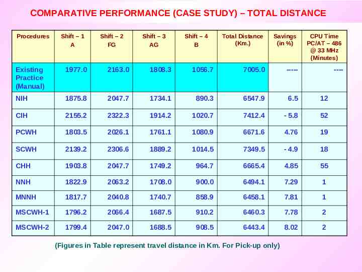
COMPARATIVE PERFORMANCE (CASE STUDY) – TOTAL DISTANCE Procedures Shift – 1 A Shift – 2 FG Shift – 3 AG Shift – 4 B Total Distance (Km.) Savings (in %) CPU Time PC/AT – 486 @ 33 MHz (Minutes) ---- Existing Practice (Manual) 1977.0 2163.0 1808.3 1056.7 7005.0 ----- NIH 1875.8 2047.7 1734.1 890.3 6547.9 6.5 12 CIH 2155.2 2322.3 1914.2 1020.7 7412.4 - 5.8 52 PCWH 1803.5 2026.1 1761.1 1080.9 6671.6 4.76 19 SCWH 2139.2 2306.6 1889.2 1014.5 7349.5 - 4.9 18 CHH 1903.8 2047.7 1749.2 964.7 6665.4 4.85 55 NNH 1822.9 2063.2 1708.0 900.0 6494.1 7.29 1 MNNH 1817.7 2040.8 1740.7 858.9 6458.1 7.81 1 MSCWH-1 1796.2 2066.4 1687.5 910.2 6460.3 7.78 2 MSCWH-2 1799.4 2047.0 1688.5 908.5 6443.4 8.02 2 (Figures in Table represent travel distance in Km. For Pick-up only)
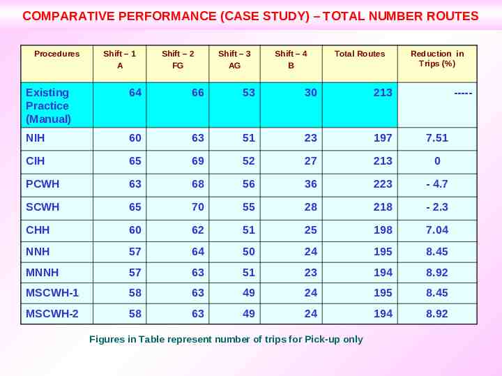
COMPARATIVE PERFORMANCE (CASE STUDY) – TOTAL NUMBER ROUTES Procedures Shift – 1 A Shift – 2 FG Shift – 3 AG Shift – 4 B Total Routes Reduction in Trips (%) Existing Practice (Manual) 64 66 53 30 213 NIH 60 63 51 23 197 7.51 CIH 65 69 52 27 213 0 PCWH 63 68 56 36 223 - 4.7 SCWH 65 70 55 28 218 - 2.3 CHH 60 62 51 25 198 7.04 NNH 57 64 50 24 195 8.45 MNNH 57 63 51 23 194 8.92 MSCWH-1 58 63 49 24 195 8.45 MSCWH-2 58 63 49 24 194 8.92 Figures in Table represent number of trips for Pick-up only -----
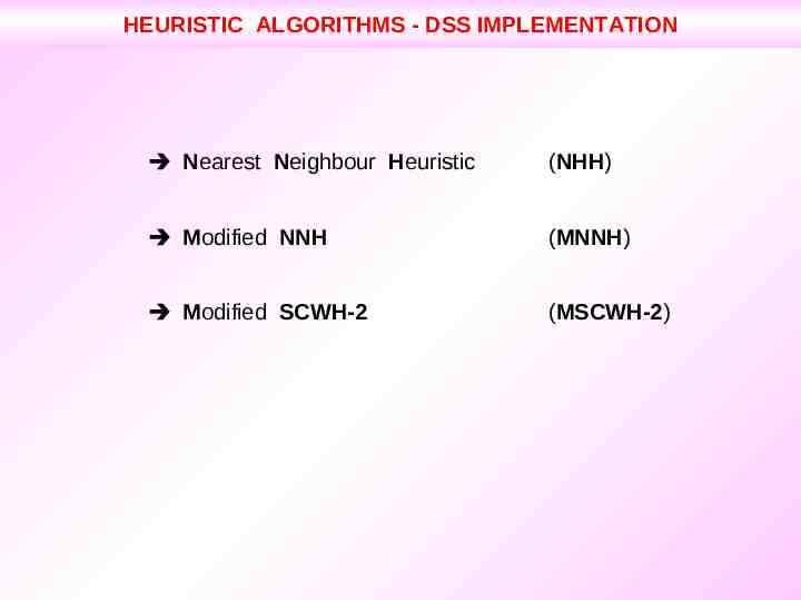
HEURISTIC ALGORITHMS - DSS IMPLEMENTATION Nearest Neighbour Heuristic (NHH) Modified NNH (MNNH) Modified SCWH-2 (MSCWH-2)
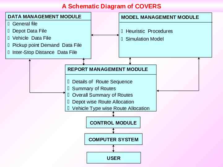
A Schematic Diagram of COVERS DATA MANAGEMENT MODULE General file Depot Data File Vehicle Data File Pickup point Demand Data File Inter-Stop Distance Data File MODEL MANAGEMENT MODULE Heuristic Procedures Simulation Model REPORT MANAGEMENT MODULE Details of Route Sequence Summary of Routes Overall Summary of Routes Depot wise Route Allocation Vehicle Type wise Route Allocation CONTROL MODULE COMPUTER SYSTEM USER