Data Modeling Patrice Koehl Department of Biological Sciences
25 Slides1.58 MB
Data Modeling Patrice Koehl Department of Biological Sciences National University of Singapore http://www.cs.ucdavis.edu/ koehl/Teaching/BL5229 [email protected]
Data Modeling Data Modeling: least squares Data Modeling: Non linear least squares Data Modeling: robust estimation
Data Modeling
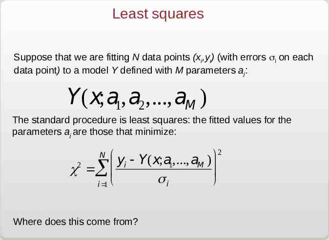
Least squares Suppose that we are fitting N data points (xi,yi) (with errors i on each data point) to a model Y defined with M parameters aj: Y(x;a1,a2,.,aM ) The standard procedure is least squares: the fitted values for the parameters aj are those that minimize: 2 æ ö yi - Y(x;a1,., aM ) 2 c å ç si ø i 1 è N Where does this come from?
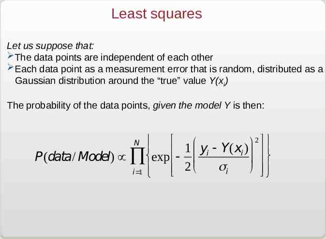
Least squares Let us suppose that: The data points are independent of each other Each data point as a measurement error that is random, distributed as a Gaussian distribution around the “true” value Y(xi) The probability of the data points, given the model Y is then: ìï é P(data/ Model) µ Õíexp ê i 1 ï î êë N 1 æ yi - Y(xi ) ö ç 2è si ø 2 ù üï úý úû ïþ
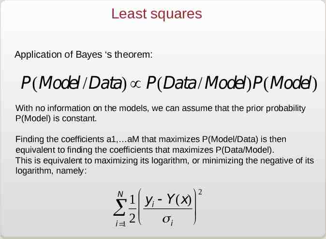
Least squares Application of Bayes ‘s theorem: P(Model /Data) µ P(Data/ Model)P(Model) With no information on the models, we can assume that the prior probability P(Model) is constant. Finding the coefficients a1, aM that maximizes P(Model/Data) is then equivalent to finding the coefficients that maximizes P(Data/Model). This is equivalent to maximizing its logarithm, or minimizing the negative of its logarithm, namely: 2 æ ö 1 yi - Y(x) å 2 çè s ø i i 1 N
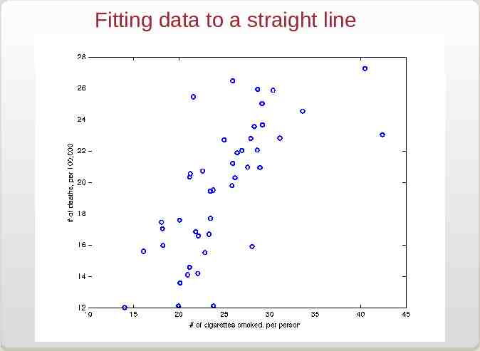
Fitting data to a straight line
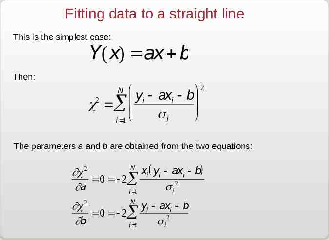
Fitting data to a straight line This is the simplest case: Y(x) ax b Then: N æ yi - axi 2 c å ç si i 1 è 2 ö b ø The parameters a and b are obtained from the two equations: N xi ( yi - axi - b) ¶c 2 0 - 2å 2 ¶a s i i 1 N ¶c 2 yi - axi - b 0 - 2å 2 ¶b s i i 1
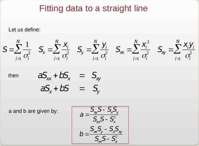
Fitting data to a straight line Let us define: N 1 S å 2 s i 1 i then N xi Sx å 2 s i 1 i N yi Sy å 2 s i 1 i xi 2 Sxx å 2 si i 1 aSxx bSx Sxy aSx bS Sy a and b are given by: N SxyS - SxSy a SxxS - Sx2 SxxSy - SxSxy b SxxS - Sx2 N xi yi Sxy å 2 si i 1
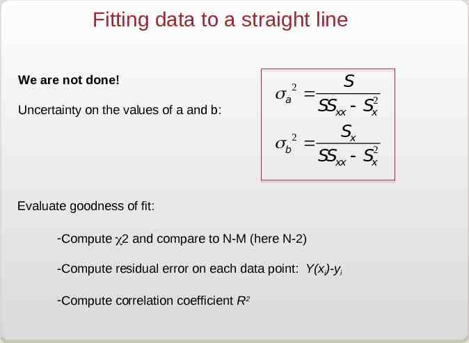
Fitting data to a straight line We are not done! Uncertainty on the values of a and b: sa sb 2 2 S SSxx - Sx2 Sx SSxx - Sx2 Evaluate goodness of fit: -Compute 2 and compare to N-M (here N-2) -Compute residual error on each data point: Y(xi)-yi -Compute correlation coefficient R2
Fitting data to a straight line
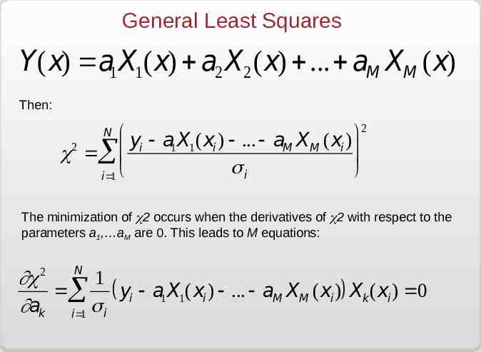
General Least Squares Y(x) a1 X1 (x) a2 X2 (x) . aM XM (x) Then: 2 æ ö yi - a1 X1 (xi ) - . - aM XM (xi ) 2 c å ç si ø i 1 è N The minimization of 2 occurs when the derivatives of 2 with respect to the parameters a1, aM are 0. This leads to M equations: ¶c 2 N 1 å ( yi - a1 X1 (xi ) - . - aM XM (xi )) Xk(xi ) 0 ¶ak i 1 s i
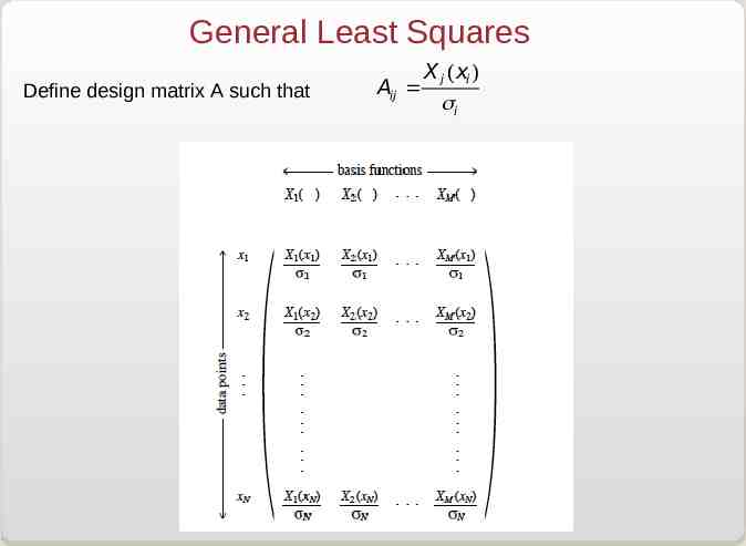
General Least Squares Define design matrix A such that Aij X j (xi ) si
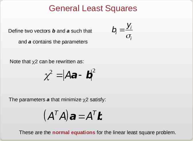
General Least Squares yi bi si Define two vectors b and a such that and a contains the parameters Note that 2 can be rewritten as: 2 2 c Aa- b The parameters a that minimize 2 satisfy: T T ( A A) a A b These are the normal equations for the linear least square problem.
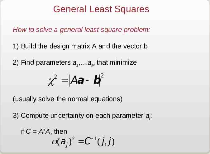
General Least Squares How to solve a general least square problem: 1) Build the design matrix A and the vector b 2) Find parameters a1, aM that minimize 2 2 c Aa- b (usually solve the normal equations) 3) Compute uncertainty on each parameter aj: if C ATA, then s(aj ) 2 C - 1 ( j, j)
Data Modeling
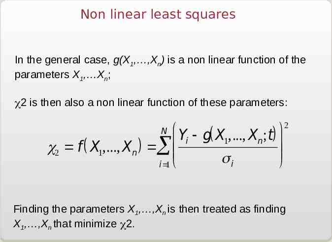
Non linear least squares In the general case, g(X1, ,Xn) is a non linear function of the parameters X1, Xn; 2 is then also a non linear function of these parameters: æ Y - g( X ,., X ;t) ö i 1 n c2 f ( X1,., Xn ) å çç si i 1 è ø N 2 Finding the parameters X1, ,Xn is then treated as finding X1, ,Xn that minimize 2.
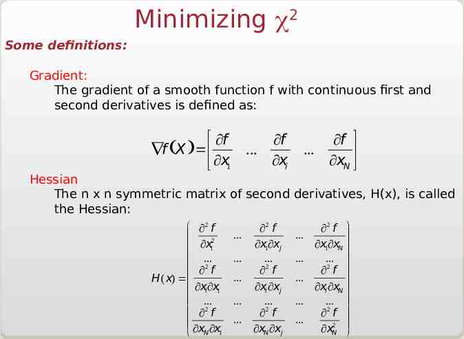
Minimizing 2 Some definitions: Gradient: The gradient of a smooth function f with continuous first and second derivatives is defined as: é ¶f Ñf (X ) ê ë ¶x1 ¶f . ¶xi ¶f ù . ¶xN úû Hessian The n x n symmetric matrix of second derivatives, H(x), is called the Hessian: æ ¶2 f ç 2 ç ¶x1 ç . ç ¶2 f H ( x) ç ç ¶xi ¶x1 ç . ç ¶2 f ç è ¶xN ¶x1 . . . . . ¶2 f ¶x1¶xj . ¶2 f ¶xi ¶xj . ¶2 f ¶xN ¶xj . . . . . ¶2 f ö ¶x1¶xN . ¶2 f ¶xi ¶xN . ¶2 f ¶xN2 ø
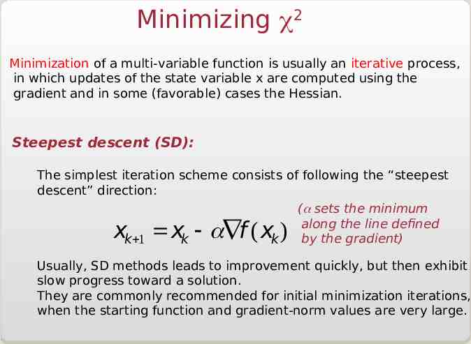
Minimizing 2 Minimization of a multi-variable function is usually an iterative process, in which updates of the state variable x are computed using the gradient and in some (favorable) cases the Hessian. Steepest descent (SD): The simplest iteration scheme consists of following the “steepest descent” direction: ( sets the minimum along the line defined by the gradient) k 1 k k x x - aÑf ( x ) Usually, SD methods leads to improvement quickly, but then exhibit slow progress toward a solution. They are commonly recommended for initial minimization iterations, when the starting function and gradient-norm values are very large.
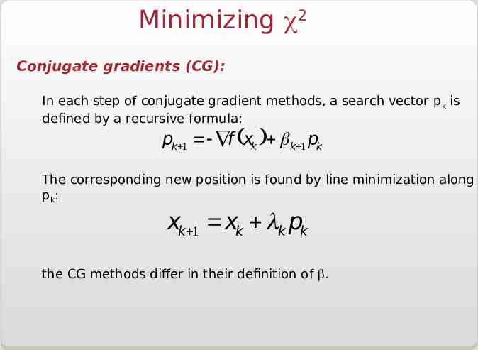
Minimizing 2 Conjugate gradients (CG): In each step of conjugate gradient methods, a search vector p k is defined by a recursive formula: pk 1 - Ñf (xk ) b k 1 pk The corresponding new position is found by line minimization along pk: xk 1 xk lk pk the CG methods differ in their definition of .
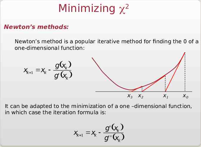
Minimizing 2 Newton’s methods: Newton’s method is a popular iterative method for finding the 0 of a one-dimensional function: xk 1 xk - g(xk ) g' (xk ) x3 x2 x1 x0 It can be adapted to the minimization of a one –dimensional function, in which case the iteration formula is: g' (xk ) xk 1 xk g' ' (xk )
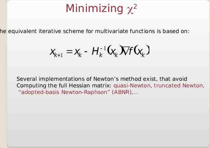
Minimizing 2 he equivalent iterative scheme for multivariate functions is based on: xk 1 xk - H -1 k (xk )Ñf (xk ) Several implementations of Newton’s method exist, that avoid Computing the full Hessian matrix: quasi-Newton, truncated Newton, “adopted-basis Newton-Raphson” (ABNR),
Data analysis and Data Modeling
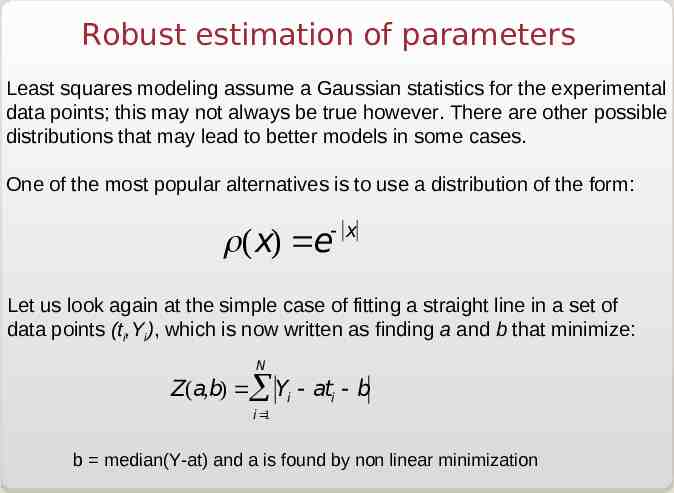
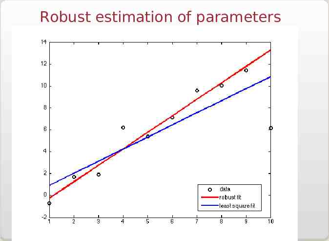
Robust estimation of parameters Least squares modeling assume a Gaussian statistics for the experimental data points; this may not always be true however. There are other possible distributions that may lead to better models in some cases. One of the most popular alternatives is to use a distribution of the form: - x r(x) e Let us look again at the simple case of fitting a straight line in a set of data points (ti,Yi), which is now written as finding a and b that minimize: N Z(a,b) å Yi - ati - b i 1 b median(Y-at) and a is found by non linear minimization
Robust estimation of parameters