ECpE Department EE653 Power distribution system modeling,

ECpE Department EE653 Power distribution system modeling, optimization and simulation Dr. Zhaoyu Wang 1113 Coover Hall, Ames, IA [email protected]

Modeling Voltage Regulators Acknowledgement: The slides are developed based in part on Distribution System Modeling and Analysis, 4th edition, William H. Kersting, CRC Press, 2017 2

Voltage Regulation The regulation of voltages is an important function on a distribution feeder. As the loads on the feeders vary, there must be some means of regulating the voltage so that every customer's voltage remains within an acceptable level. Common methods of regulating the voltage are the application of steptype voltage regulators, load tap changing (LTC) transformers, and shunt capacitors. A step-voltage regulator is basically an autotransformer with a LTC mechanism on the “series” winding. The voltage change is obtained by changing the number of turns (tap changes) of the series winding of the autotransformer. An autotransformer can be visualized as a two-winding transformer with a solid connection between a terminal on the primary side of the transformer and a terminal on the secondary. 3 ECpE Department

Standard Voltage Ratings The American National Standards Institute (ANSI) standard ANSI C84.1-1995 for “Electric Power Systems and Equipment Voltage Ratings (60 Hertz)” provides the following definitions for system voltage terms [1]: o System voltage: The root mean square (rms) phasor voltage of a portion of an alternating current electric system. Each system voltage pertains to a portion of the system that is bounded by transformers or utilization equipment. o Nominal system voltage: The voltage by which a portion of the system is designated and to which certain operating characteristics of the system are related. Each nominal system voltage pertains to a portion of the system bounded by transformers or utilization equipment. o Maximum system voltage: The highest system voltage that occurs under normal operating conditions, and the highest system voltage for which equipment and other components are designed for satisfactory continuous operation without derating of any kind. o Service voltage: The voltage at the point where the electrical system of the supplier and the electrical system of the user are connected. o Utilization voltage: The voltage at the line terminals of utilization equipment. o Nominal utilization voltage: The voltage rating of certain utilization equipment used on the system. [1] American Nation Standard for Electric Power—Systems and Equipment Voltage Ratings (60 Hertz), ANSI C84.1-1995, National Electrical Manufacturers 4 Association, Rosslyn, VA, 1996. ECpE Department

Standard Voltage Ratings The ANSI standard specifies two voltage ranges. An over simplification of the voltage ranges is Range A: Electric supply systems shall be so designated and operated such that most service voltages will be within the limits specified for range A. The occurrence of voltages outside of these limits should be infrequent. Range B: Voltages above and below range A. When these voltages occur, corrective measures shall be undertaken within a reasonable time to improve voltages to meet range A. For a normal three-wire 120/240 V service to a user, the range A and range B voltages are Range A: o Nominal utilization voltage 115 V o Maximum utilization and service voltage 126 V o Minimum service voltage 114 V o Minimum utilization voltage 110 V Range B: o Nominal utilization voltage 115 V o Maximum utilization and service voltage 127 V o Minimum service voltage 110 V o Minimum utilization voltage 107 V 5 ECpE Department

Standard Voltage Ratings These ANSI standards give the distribution engineer a range of “normal steady-state” voltages (range A) and a range of “emergency steady-state” voltages (range B) that must be supplied to all users. In addition to the acceptable voltage magnitude ranges, the ANSI standard recommends that the “electric supply systems should be designed and operated to limit the maximum voltage unbalance to 3 percent when measured at the electric-utility revenue meter under a no-load condition.” Voltage unbalance is defined as 𝑉𝑜𝑙𝑡𝑎𝑔𝑒𝑢𝑛𝑏𝑎𝑙𝑎𝑛𝑐𝑒 𝑀𝑎𝑥 . 𝑑𝑒𝑣𝑖𝑎𝑡𝑖𝑜𝑛 𝑓𝑟𝑜𝑚 𝑎𝑣𝑒𝑟𝑎𝑔𝑒 𝑣𝑜𝑙𝑡𝑎𝑔𝑒 1 00 % 𝐴𝑣𝑒𝑟𝑎𝑔𝑒 𝑣𝑜𝑙𝑡𝑎𝑔𝑒 (1) The task for the distribution engineer is to design and operate the distribution system so that under normal steady-state conditions the voltages at the meters of all users will lie within Range A and that the voltage unbalance will not exceed 3%. A common device used to maintain system voltages is the step-voltage regulator. Step-voltage regulators can be single phase or three phase. Single-phase regulators can be connected in wye, delta, or open delta, in addition to operating as a single-phase device. The regulators and their 6 controls allow the voltage output to vary as the load varies. ECpE Department

Standard Voltage Ratings A common device used to maintain system voltages is the step-voltage regulator. Step-voltage regulators can be single phase or three phase. Single-phase regulators can be connected in wye, delta, or open delta, in addition to operating as a single-phase device. The regulators and their controls allow the voltage output to vary as the load varies. A step-voltage regulator is basically an autotransformer with a LTC mechanism on the “series” winding. The voltage change is obtained by changing the number of turns (tap changes) of the series winding of the autotransformer. An autotransformer can be visualized as a two-winding transformer with a solid connection between a terminal on the primary side of the transformer and a terminal on the secondary. Before proceeding to the autotransformer, a review of two-transformer theory and the development of generalized constants will be presented. 7

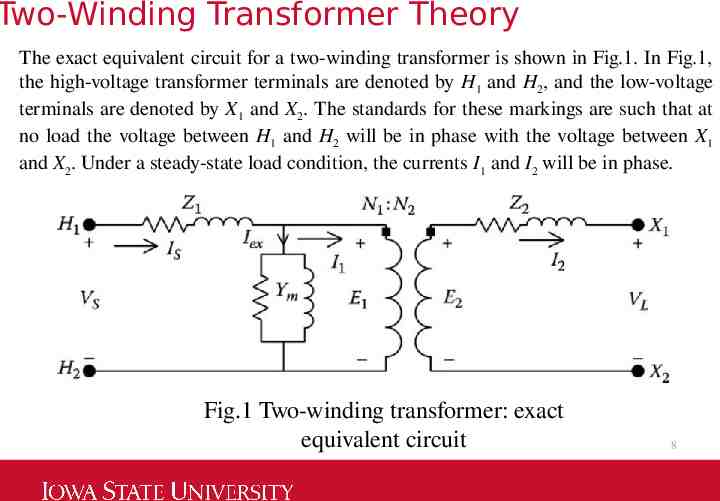
Two-Winding Transformer Theory The exact equivalent circuit for a two-winding transformer is shown in Fig.1. In Fig.1, the high-voltage transformer terminals are denoted by H1 and H2, and the low-voltage terminals are denoted by X1 and X2. The standards for these markings are such that at no load the voltage between H1 and H2 will be in phase with the voltage between X1 and X2. Under a steady-state load condition, the currents I1 and I2 will be in phase. Fig.1 Two-winding transformer: exact equivalent circuit 8

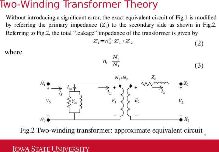
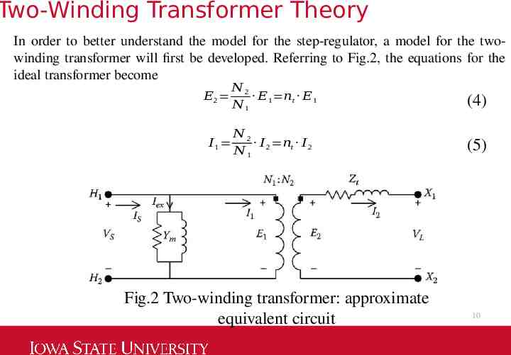
Two-Winding Transformer Theory Without introducing a significant error, the exact equivalent circuit of Fig.1 is modified by referring the primary impedance (Z1) to the secondary side as shown in Fig.2. Referring to Fig.2, the total “leakage” impedance of the transformer is given by 𝑍 t 𝑛 2𝑡 𝑍 1 𝑍 2 where 𝑛t 𝑁2 𝑁1 (2) (3) Fig.2 Two-winding transformer: approximate equivalent circuit 9

Two-Winding Transformer Theory In order to better understand the model for the step-regulator, a model for the twowinding transformer will first be developed. Referring to Fig.2, the equations for the ideal transformer become 𝐸2 𝑁2 𝐸1 𝑛 t 𝐸 1 𝑁1 (4) 𝐼1 𝑁2 𝐼 𝑛t 𝐼 2 𝑁1 2 (5) Fig.2 Two-winding transformer: approximate equivalent circuit 10

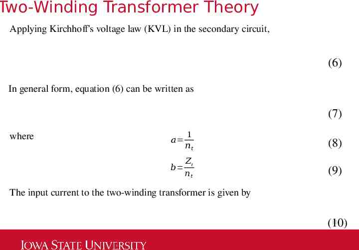
Two-Winding Transformer Theory Applying Kirchhoff's voltage law (KVL) in the secondary circuit, (6) In general form, equation (6) can be written as (7) where 𝑎 1 𝑛𝑡 (8) 𝑏 𝑍t 𝑛𝑡 (9) The input current to the two-winding transformer is given by 11 (10)

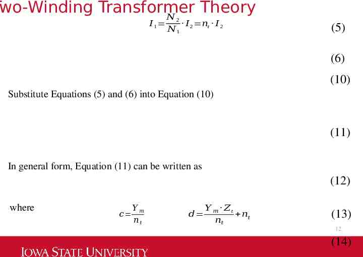
Two-Winding Transformer Theory 𝑁 𝐼1 2 𝑁1 𝐼 2 𝑛t 𝐼 2 (5) (6) (10) Substitute Equations (5) and (6) into Equation (10) (11) In general form, Equation (11) can be written as (12) where 𝑐 𝑌𝑚 𝑛𝑡 𝑑 𝑌 𝑚 𝑍t 𝑛𝑡 𝑛𝑡 (13) 12 (14)

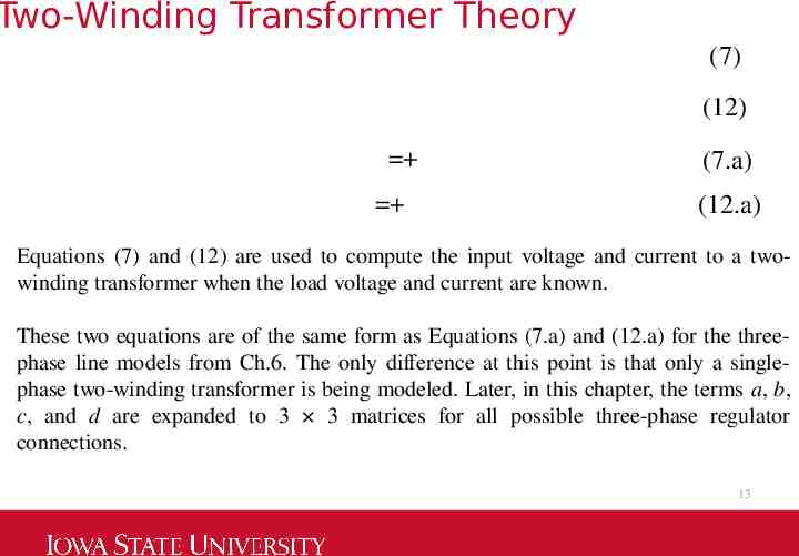
Two-Winding Transformer Theory (7) (12) (7.a) (12.a) Equations (7) and (12) are used to compute the input voltage and current to a twowinding transformer when the load voltage and current are known. These two equations are of the same form as Equations (7.a) and (12.a) for the threephase line models from Ch.6. The only difference at this point is that only a singlephase two-winding transformer is being modeled. Later, in this chapter, the terms a, b, c, and d are expanded to 3 3 matrices for all possible three-phase regulator connections. 13

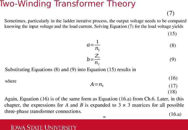
Two-Winding Transformer Theory (7) Sometimes, particularly in the ladder iterative process, the output voltage needs to be computed knowing the input voltage and the load current. Solving Equation (7) for the load voltage yields (15) 𝑎 1 𝑛𝑡 (8) 𝑏 𝑍t 𝑛𝑡 (9) Substituting Equations (8) and (9) into Equation (15) results in (16) 𝐴 𝑛𝑡 (17) (18) Again, Equation (16) is of the same form as Equation (16.a) from Ch.6. Later, in this 14 chapter, the expressions for A and B is expanded to 3 3 matrices for all possible three-phase transformer connections. (16.a) where

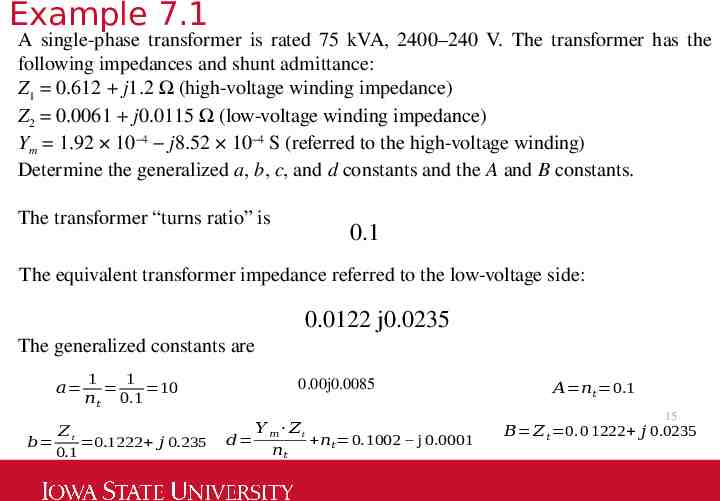
Example 7.1 A single-phase transformer is rated 75 kVA, 2400–240 V. The transformer has the following impedances and shunt admittance: Z1 0.612 j1.2 Ω (high-voltage winding impedance) Z2 0.0061 j0.0115 Ω (low-voltage winding impedance) Ym 1.92 10 4 j8.52 10 4 S (referred to the high-voltage winding) Determine the generalized a, b, c, and d constants and the A and B constants. The transformer “turns ratio” is 0.1 The equivalent transformer impedance referred to the low-voltage side: 0.0122 j0.0235 The generalized constants are 𝑎 𝑏 1 1 10 𝑛𝑡 0.1 𝑍t 0.1222 𝑗 0.235 0.1 0.00j0.0085 𝑌 𝑚 𝑍t 𝑑 𝑛𝑡 0.1002 j 0.0001 𝑛𝑡 𝐴 𝑛𝑡 0.1 15 𝐵 𝑍 𝑡 0. 0 1222 𝑗 0.0235

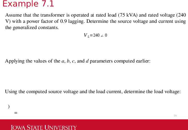
Example 7.1 Assume that the transformer is operated at rated load (75 kVA) and rated voltage (240 V) with a power factor of 0.9 lagging. Determine the source voltage and current using the generalized constants. 𝑉 𝐿 240 0 Applying the values of the a, b, c, and d parameters computed earlier: Using the computed source voltage and the load current, determine the load voltage: ) 16

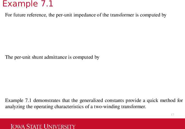
Example 7.1 For future reference, the per-unit impedance of the transformer is computed by The per-unit shunt admittance is computed by Example 7.1 demonstrates that the generalized constants provide a quick method for analyzing the operating characteristics of a two-winding transformer. 17

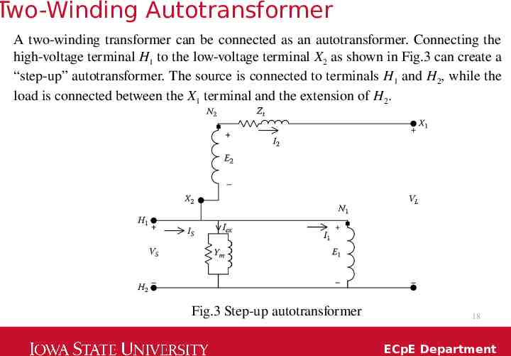
Two-Winding Autotransformer A two-winding transformer can be connected as an autotransformer. Connecting the high-voltage terminal H1 to the low-voltage terminal X2 as shown in Fig.3 can create a “step-up” autotransformer. The source is connected to terminals H1 and H2, while the load is connected between the X1 terminal and the extension of H2. Fig.3 Step-up autotransformer 18 ECpE Department

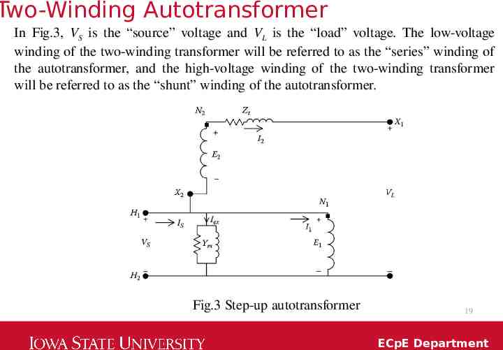
Two-Winding Autotransformer In Fig.3, VS is the “source” voltage and VL is the “load” voltage. The low-voltage winding of the two-winding transformer will be referred to as the “series” winding of the autotransformer, and the high-voltage winding of the two-winding transformer will be referred to as the “shunt” winding of the autotransformer. Fig.3 Step-up autotransformer 19 ECpE Department

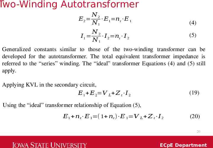
Two-Winding Autotransformer 𝐸2 𝑁2 𝐸1 𝑛 t 𝐸 1 𝑁1 𝐼1 𝑁2 𝐼 2 𝑛t 𝐼 2 𝑁1 (4) (5) Generalized constants similar to those of the two-winding transformer can be developed for the autotransformer. The total equivalent transformer impedance is referred to the “series” winding. The “ideal” transformer Equations (4) and (5) still apply. Applying KVL in the secondary circuit, 𝐸1 𝐸 2 𝑉 𝐿 𝑍 t 𝐼 2 (19) Using the “ideal” transformer relationship of Equation (5), 𝐸1 𝑛 t 𝐸 1 ( 1 𝑛t ) 𝐸 1 𝑉 𝐿 𝑍 t 𝐼 2 (20) 20 ECpE Department

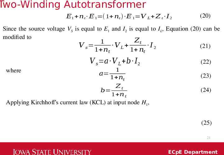
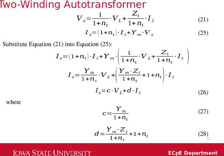
Two-Winding Autotransformer 𝐸1 𝑛 t 𝐸 1 ( 1 𝑛t ) 𝐸 1 𝑉 𝐿 𝑍 t 𝐼 2 (20) Since the source voltage VS is equal to E1 and I2 is equal to IL, Equation (20) can be modified to 𝑍𝑡 1 𝑉 𝑠 𝑉 𝐿 𝐼2 (21) 1 𝑛𝑡 1 𝑛 𝑡 𝑉 𝑠 𝑎 𝑉 𝐿 𝑏 𝐼 2 where (22) 1 𝑎 1 𝑛𝑡 (23) 𝑍𝑡 1 𝑛 𝑡 (24) 𝑏 Applying Kirchhoff's current law (KCL) at input node H1, (25) 21 ECpE Department

Two-Winding Autotransformer 𝑍𝑡 1 𝑉 𝑠 𝑉 𝐿 𝐼2 1 𝑛 𝑡 1 𝑛𝑡 (21) 𝐼 𝑠 ( 1 𝑛𝑡 ) 𝐼 2 𝑌 𝑚 𝑉 𝑠 (25) Substitute Equation (21) into Equation (25): ( ( 𝐼 𝑠 ( 1 𝑛𝑡 ) 𝐼 2 𝑌 𝑚 𝐼 𝑠 𝑍𝑡 1 𝑉 𝐿 𝐼 1 𝑛𝑡 1 𝑛𝑡 2 ) 𝑌𝑚 𝑌 𝑚 𝑍𝑡 𝑉 𝐿 1 𝑛𝑡 𝐼 2 1 𝑛 𝑡 1 𝑛𝑡 𝐼 𝑠 𝑐 𝑉 𝐿 𝑑 𝐼 2 where ) (26) 𝑌𝑚 1 𝑛𝑡 (27) 𝑌 𝑚 𝑍𝑡 𝑑 1 𝑛𝑡 1 𝑛𝑡 (28) 𝑐 22 ECpE Department

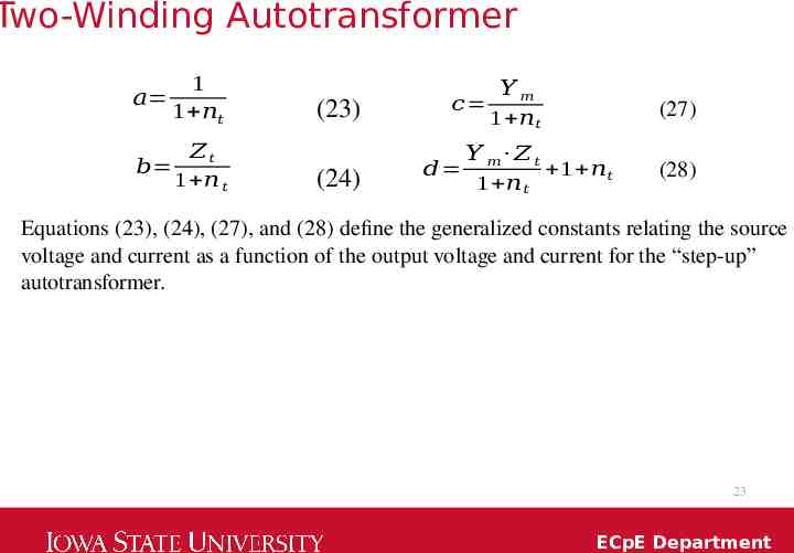
Two-Winding Autotransformer 𝑎 1 1 𝑛𝑡 𝑍𝑡 𝑏 1 𝑛 𝑡 (23) (24) 𝑌𝑚 𝑐 1 𝑛𝑡 𝑑 (27) 𝑌 𝑚 𝑍𝑡 1 𝑛𝑡 1 𝑛𝑡 (28) Equations (23), (24), (27), and (28) define the generalized constants relating the source voltage and current as a function of the output voltage and current for the “step-up” autotransformer. 23 ECpE Department

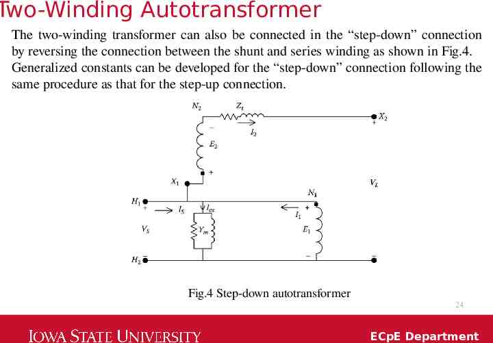
Two-Winding Autotransformer The two-winding transformer can also be connected in the “step-down” connection by reversing the connection between the shunt and series winding as shown in Fig.4. Generalized constants can be developed for the “step-down” connection following the same procedure as that for the step-up connection. Fig.4 Step-down autotransformer 24 ECpE Department

Two-Winding Autotransformer Applying KVL in the secondary circuit, 𝐸1 𝐸 2 𝑉 𝐿 𝑍 t 𝐼 2 (29) 𝑁2 𝐼 𝑛t 𝐼 2 𝑁1 2 (5) 𝐼1 Using the “ideal” transformer relationship of Equation (5), 𝐸1 𝑛t 𝐸1 𝑉 𝐿 𝑍 t 𝐼 2 (30) 25 ECpE Department

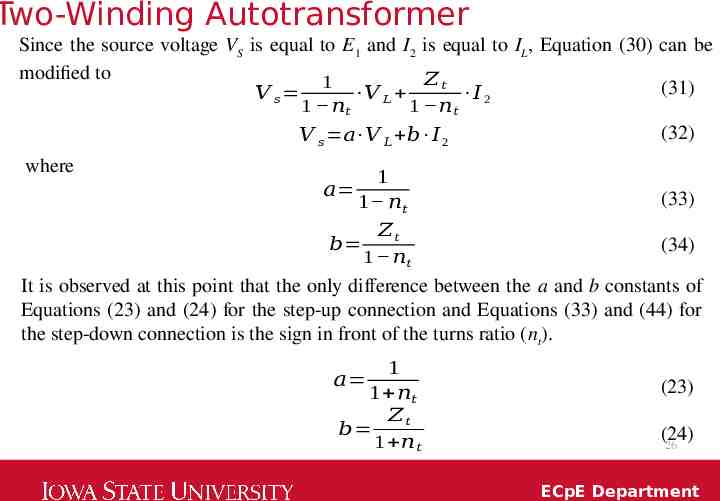
Two-Winding Autotransformer Since the source voltage VS is equal to E1 and I2 is equal to IL, Equation (30) can be modified to 𝑍𝑡 1 (31) 𝑉 𝑠 𝑉 𝐿 𝐼2 1 𝑛𝑡 1 𝑛𝑡 𝑉 𝑠 𝑎 𝑉 𝐿 𝑏 𝐼 2 where 𝑎 1 1 𝑛𝑡 𝑏 𝑍𝑡 1 𝑛𝑡 (32) (33) (34) It is observed at this point that the only difference between the a and b constants of Equations (23) and (24) for the step-up connection and Equations (33) and (44) for the step-down connection is the sign in front of the turns ratio (nt). 𝑎 1 1 𝑛𝑡 𝑏 𝑍𝑡 1 𝑛 𝑡 (23) (24) 26 ECpE Department

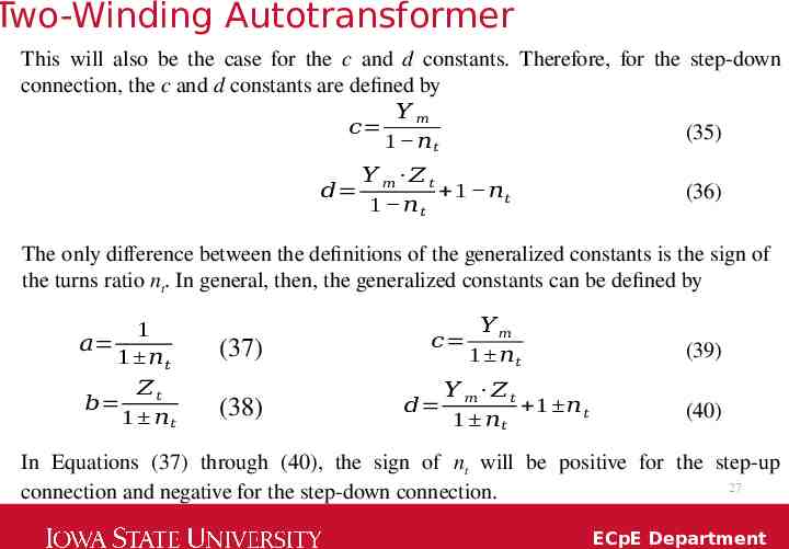
Two-Winding Autotransformer This will also be the case for the c and d constants. Therefore, for the step-down connection, the c and d constants are defined by 𝑌𝑚 𝑐 1 𝑛𝑡 (35) 𝑌 𝑚 𝑍𝑡 𝑑 1 𝑛𝑡 1 𝑛 𝑡 (36) The only difference between the definitions of the generalized constants is the sign of the turns ratio nt. In general, then, the generalized constants can be defined by 1 𝑎 1 𝑛 𝑡 𝑏 𝑍𝑡 1 𝑛𝑡 (37) (38) 𝑌𝑚 𝑐 1 𝑛𝑡 𝑑 𝑌 𝑚 𝑍𝑡 1 𝑛 𝑡 1 𝑛𝑡 (39) (40) In Equations (37) through (40), the sign of nt will be positive for the step-up 27 connection and negative for the step-down connection. ECpE Department

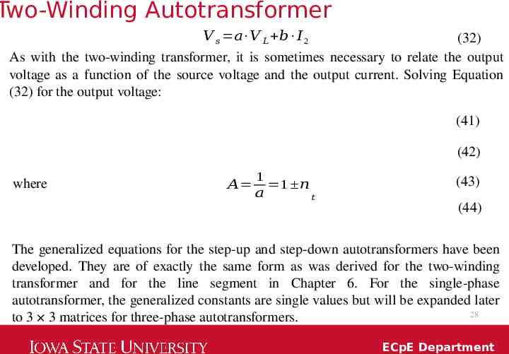
Two-Winding Autotransformer 𝑉 𝑠 𝑎 𝑉 𝐿 𝑏 𝐼 2 (32) As with the two-winding transformer, it is sometimes necessary to relate the output voltage as a function of the source voltage and the output current. Solving Equation (32) for the output voltage: (41) (42) where 𝐴 1 1 𝑛 𝑎 𝑡 (43) (44) The generalized equations for the step-up and step-down autotransformers have been developed. They are of exactly the same form as was derived for the two-winding transformer and for the line segment in Chapter 6. For the single-phase autotransformer, the generalized constants are single values but will be expanded later 28 to 3 3 matrices for three-phase autotransformers. ECpE Department

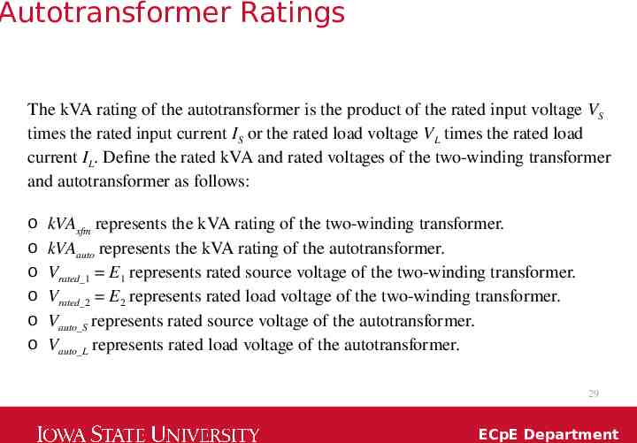
Autotransformer Ratings The kVA rating of the autotransformer is the product of the rated input voltage VS times the rated input current IS or the rated load voltage VL times the rated load current IL. Define the rated kVA and rated voltages of the two-winding transformer and autotransformer as follows: o o o o o o kVAxfm represents the kVA rating of the two-winding transformer. kVAauto represents the kVA rating of the autotransformer. Vrated 1 E1 represents rated source voltage of the two-winding transformer. Vrated 2 E2 represents rated load voltage of the two-winding transformer. Vauto S represents rated source voltage of the autotransformer. Vauto L represents rated load voltage of the autotransformer. 29 ECpE Department

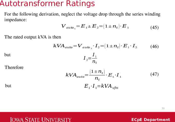
Autotransformer Ratings For the following derivation, neglect the voltage drop through the series winding impedance: 𝑉 𝑎𝑢𝑡𝑜 𝐸 1 𝐸 2 ( 1 𝑛𝑡 ) 𝐸 1 (45) 𝐿 The rated output kVA is then 𝑘𝑉𝐴𝑎𝑢𝑡𝑜 𝑉 𝑎𝑢𝑡𝑜 𝐼 2 ( 1 𝑛𝑡 ) 𝐸1 𝐼 2 𝐿 but 𝐼1 𝐼 2 𝑛𝑡 Therefore 𝑘𝑉𝐴𝑎𝑢𝑡𝑜 but (46) ( 1 𝑛𝑡 ) 𝑛𝑡 𝐸1 𝐼 1 (47) 𝐸1 𝐼 1 𝑘𝑉𝐴 𝑥𝑓𝑚 30 ECpE Department

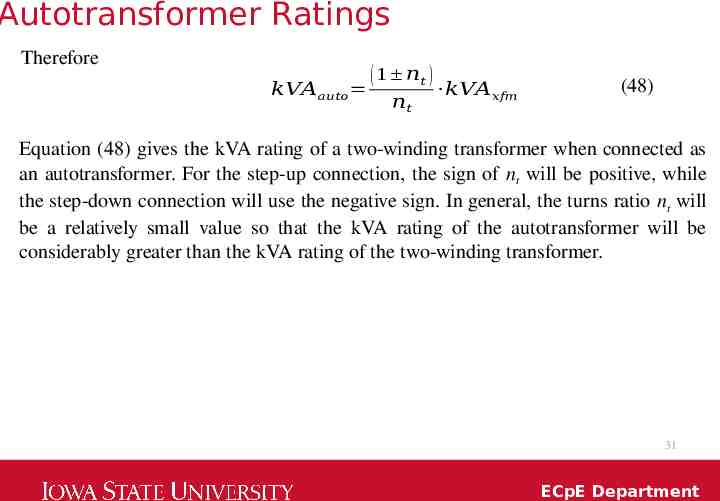
Autotransformer Ratings Therefore 𝑘𝑉𝐴𝑎𝑢𝑡𝑜 ( 1 𝑛𝑡 ) 𝑛𝑡 𝑘𝑉𝐴𝑥𝑓𝑚 (48) Equation (48) gives the kVA rating of a two-winding transformer when connected as an autotransformer. For the step-up connection, the sign of nt will be positive, while the step-down connection will use the negative sign. In general, the turns ratio nt will be a relatively small value so that the kVA rating of the autotransformer will be considerably greater than the kVA rating of the two-winding transformer. 31 ECpE Department

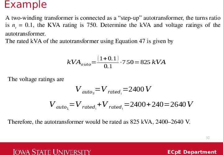
Example A two-winding transformer is connected as a “step-up” autotransformer, the turns ratio is nt 0.1, the KVA rating is 750. Determine the kVA and voltage ratings of the autotransformer. The rated kVA of the autotransformer using Equation 47 is given by 𝑘𝑉𝐴𝑎𝑢𝑡𝑜 ( 1 0.1 ) 7 50 825 𝑘𝑉𝐴 0.1 The voltage ratings are 𝑉 𝑎𝑢𝑡𝑜 𝑉 𝑟𝑎𝑡𝑒𝑑 2400 𝑉 𝑆 1 𝑉 𝑎𝑢𝑡𝑜 𝑉 𝑟𝑎𝑡𝑒𝑑 𝑉 𝑟𝑎𝑡𝑒𝑑 2400 240 2640 𝑉 𝐿 1 1 Therefore, the autotransformer would be rated as 825 kVA, 2400–2640 V. 32 ECpE Department

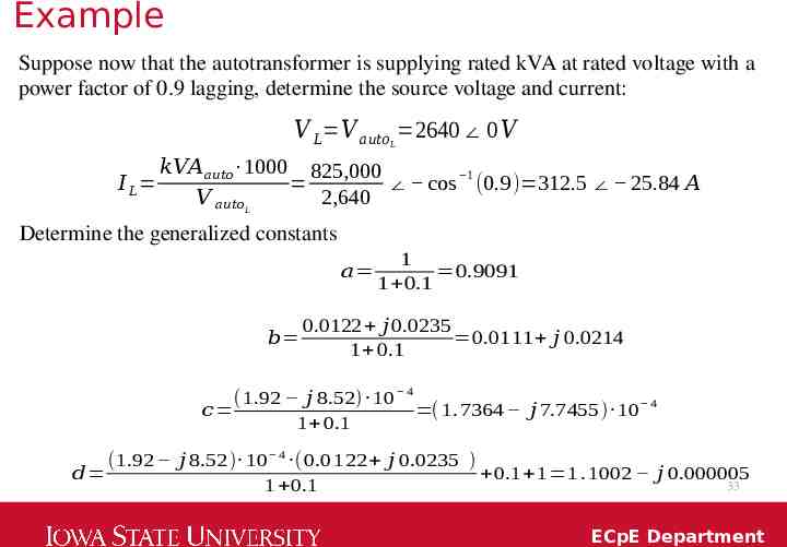
Example Suppose now that the autotransformer is supplying rated kVA at rated voltage with a power factor of 0.9 lagging, determine the source voltage and current: 𝑉 𝐿 𝑉 𝑎𝑢𝑡𝑜 2640 0 𝑉 𝐿 𝑘𝑉𝐴𝑎𝑢𝑡𝑜 1000 825,000 1 𝐼 𝐿 cos (0.9) 312.5 25.84 𝐴 𝑉 𝑎𝑢𝑡𝑜 2,640 𝐿 Determine the generalized constants 𝑎 𝑏 1 0.9091 1 0.1 0.0122 𝑗 0.0235 0.0111 𝑗 0.0214 1 0.1 (1.92 𝑗 8.52) 10 4 𝑐 ( 1.7364 𝑗 7.7455) 10 4 1 0.1 (1.92 𝑗 8.52) 10 4 (0.0 122 𝑗 0.0235 ) 𝑑 0.1 1 1 .1002 𝑗 0.000005 33 1 0.1 ECpE Department

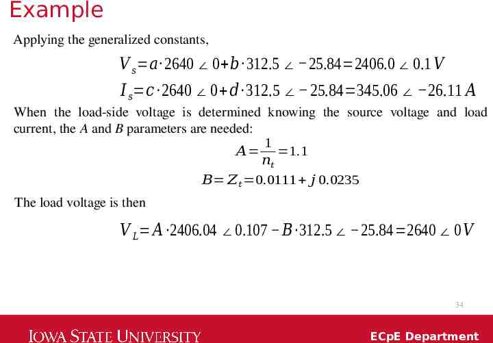
Example Applying the generalized constants, 𝑉 𝑠 𝑎 2640 0 𝑏 312.5 25.84 2406.0 0.1 𝑉 𝐼 𝑠 𝑐 2640 0 𝑑 312.5 25.84 345.06 26.11 𝐴 When the load-side voltage is determined knowing the source voltage and load current, the A and B parameters are needed: 1 𝐴 1.1 𝑛𝑡 𝐵 𝑍 𝑡 0.0111 𝑗 0.0235 The load voltage is then 𝑉 𝐿 𝐴 2406.04 0.107 𝐵 312.5 25.84 2640 0 𝑉 34 ECpE Department

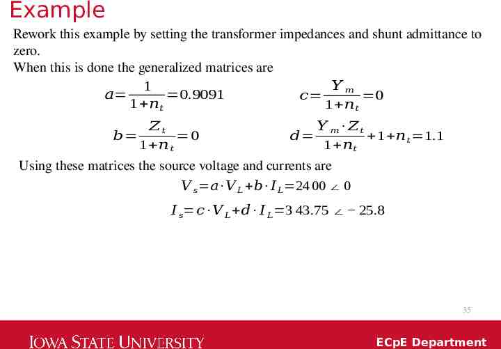
Example Rework this example by setting the transformer impedances and shunt admittance to zero. When this is done the generalized matrices are 𝑌𝑚 1 𝑎 0.9091 𝑐 0 1 𝑛𝑡 1 𝑛𝑡 𝑍𝑡 𝑏 0 1 𝑛 𝑡 𝑌 𝑚 𝑍𝑡 𝑑 1 𝑛𝑡 1.1 1 𝑛𝑡 Using these matrices the source voltage and currents are 𝑉 𝑠 𝑎 𝑉 𝐿 𝑏 𝐼 𝐿 24 00 0 𝐼 𝑠 𝑐 𝑉 𝐿 𝑑 𝐼 𝐿 3 43.75 25.8 35 ECpE Department

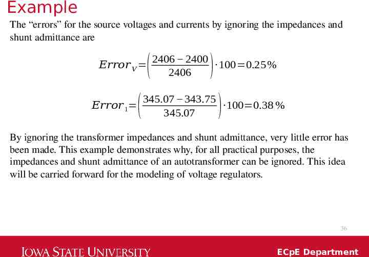
Example The “errors” for the source voltages and currents by ignoring the impedances and shunt admittance are ( 𝐸𝑟𝑟𝑜𝑟 𝑉 𝐸𝑟𝑟𝑜𝑟 1 ( 2406 2400 100 0.25 % 2406 ) 345.07 343.75 100 0.38 % 345.07 ) By ignoring the transformer impedances and shunt admittance, very little error has been made. This example demonstrates why, for all practical purposes, the impedances and shunt admittance of an autotransformer can be ignored. This idea will be carried forward for the modeling of voltage regulators. 36 ECpE Department

Example In this section, the equivalent circuit of an autotransformer has been developed for the “raise” and “lower” connections. These equivalent circuits included the series impedance and shunt admittance. If a detailed analysis of the autotransformer is desired, the series impedance and shunt admittance should be included. However, it has been shown in Example that these values are very small, and when the autotransformer is to be a component of a system, very little error will be made by neglecting both the series impedance and shunt admittance of the equivalent circuit. 37 ECpE Department

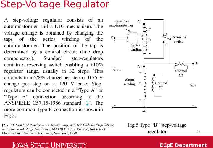
Step-Voltage Regulator A step-voltage regulator consists of an autotransformer and a LTC mechanism. The voltage change is obtained by changing the taps of the series winding of the autotransformer. The position of the tap is determined by a control circuit (line drop compensator). Standard step-regulators contain a reversing switch enabling a 10% regulator range, usually in 32 steps. This amounts to a 5/8% change per step or 0.75 V change per step on a 120 V base. Stepregulators can be connected in a “Type A” or “Type B” connection according to the ANSI/IEEE C57.15-1986 standard [2]. The more common Type B connection is shown in Fig.5. [2] IEEE Standard Requirements, Terminology, and Test Code for Step-Voltage and Induction-Voltage Regulators, ANSI/IEEE C57.15-1986, Institute of Electrical and Electronic Engineers, New York, 1988 Fig.5 Type “B” step-voltage regulator 38 ECpE Department

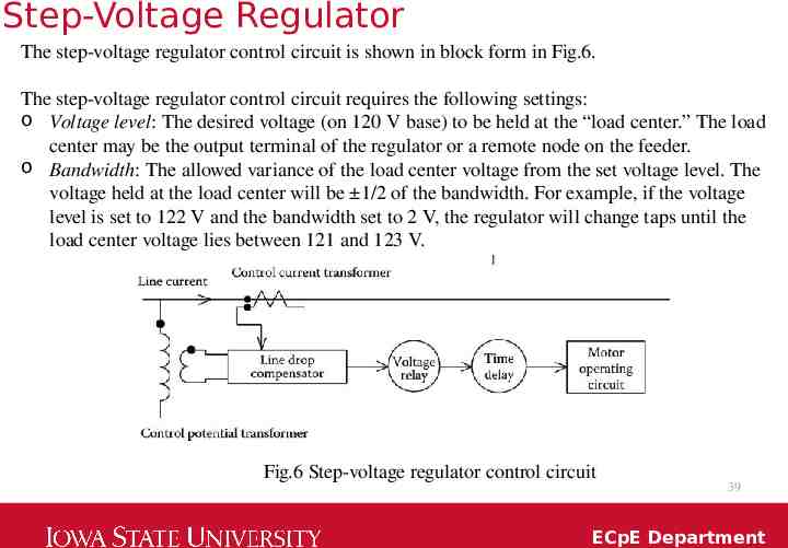
Step-Voltage Regulator The step-voltage regulator control circuit is shown in block form in Fig.6. The step-voltage regulator control circuit requires the following settings: o Voltage level: The desired voltage (on 120 V base) to be held at the “load center.” The load center may be the output terminal of the regulator or a remote node on the feeder. o Bandwidth: The allowed variance of the load center voltage from the set voltage level. The voltage held at the load center will be 1/2 of the bandwidth. For example, if the voltage level is set to 122 V and the bandwidth set to 2 V, the regulator will change taps until the load center voltage lies between 121 and 123 V. Fig.6 Step-voltage regulator control circuit 39 ECpE Department

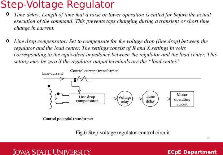
Step-Voltage Regulator o Time delay: Length of time that a raise or lower operation is called for before the actual execution of the command. This prevents taps changing during a transient or short time change in current. o Line drop compensator: Set to compensate for the voltage drop (line drop) between the regulator and the load center. The settings consist of R and X settings in volts corresponding to the equivalent impedance between the regulator and the load center. This setting may be zero if the regulator output terminals are the “load center.” Fig.6 Step-voltage regulator control circuit 40 ECpE Department

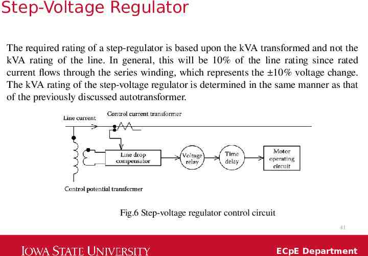
Step-Voltage Regulator The required rating of a step-regulator is based upon the kVA transformed and not the kVA rating of the line. In general, this will be 10% of the line rating since rated current flows through the series winding, which represents the 10% voltage change. The kVA rating of the step-voltage regulator is determined in the same manner as that of the previously discussed autotransformer. Fig.6 Step-voltage regulator control circuit 41 ECpE Department

Single-Phase Step-Voltage Regulator Because the series impedance and shunt admittance values of step-voltage regulators are so small, they will be neglected in the following equivalent circuits. It should be pointed out, however, that if it is desired to include the impedance and admittance, they can be incorporated into the following equivalent circuits in the same way they were originally modeled in the autotransformer equivalent circuit. 42 ECpE Department

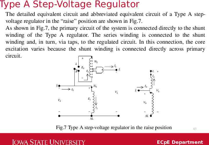
Type A Step-Voltage Regulator The detailed equivalent circuit and abbreviated equivalent circuit of a Type A stepvoltage regulator in the “raise” position are shown in Fig.7. As shown in Fig.7, the primary circuit of the system is connected directly to the shunt winding of the Type A regulator. The series winding is connected to the shunt winding and, in turn, via taps, to the regulated circuit. In this connection, the core excitation varies because the shunt winding is connected directly across primary circuit. Fig.7 Type A step-voltage regulator in the raise position 43 ECpE Department

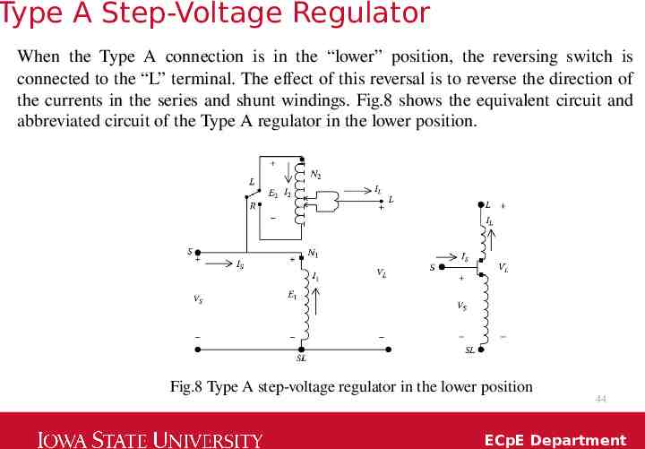
Type A Step-Voltage Regulator When the Type A connection is in the “lower” position, the reversing switch is connected to the “L” terminal. The effect of this reversal is to reverse the direction of the currents in the series and shunt windings. Fig.8 shows the equivalent circuit and abbreviated circuit of the Type A regulator in the lower position. Fig.8 Type A step-voltage regulator in the lower position 44 ECpE Department

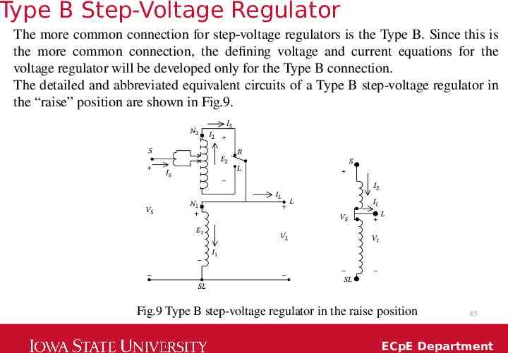
Type B Step-Voltage Regulator The more common connection for step-voltage regulators is the Type B. Since this is the more common connection, the defining voltage and current equations for the voltage regulator will be developed only for the Type B connection. The detailed and abbreviated equivalent circuits of a Type B step-voltage regulator in the “raise” position are shown in Fig.9. Fig.9 Type B step-voltage regulator in the raise position 45 ECpE Department

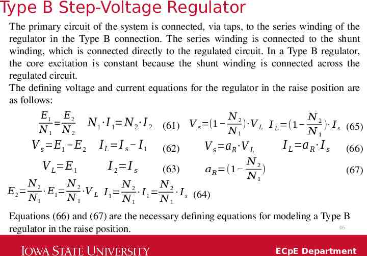
Type B Step-Voltage Regulator The primary circuit of the system is connected, via taps, to the series winding of the regulator in the Type B connection. The series winding is connected to the shunt winding, which is connected directly to the regulated circuit. In a Type B regulator, the core excitation is constant because the shunt winding is connected across the regulated circuit. The defining voltage and current equations for the regulator in the raise position are as follows: 𝐸1 𝐸 2 𝑁1 𝑁2 𝐸2 𝑁 𝑁 𝑁 1 𝐼 1 𝑁 2 𝐼 2 (61) 𝑉 𝑠 (1 2 ) 𝑉 𝐿 𝐼 𝐿 (1 2 ) 𝐼 s (65) 𝑁1 𝑁 𝑉 𝑠 𝐸1 𝐸 2 𝐼 𝐿 𝐼 𝑠 𝐼 1 𝑉 𝐿 𝐸 1 𝐼 2 𝐼 𝑠 𝑁2 𝑁2 𝐸 1 𝑉 𝐿 𝑁1 𝑁1 1 (62) 𝑉 𝑠 𝑎𝑅 𝑉 𝐿 𝑁2 𝑎 𝑅 (1 ) 𝑁1 (63) 𝑁2 𝑁2 𝐼1 𝐼 𝐼 𝑁 1 1 𝑁 1 s (64) 𝐼 𝐿 𝑎 𝑅 𝐼 𝑠 (66) (67) Equations (66) and (67) are the necessary defining equations for modeling a Type B 46 regulator in the raise position. ECpE Department

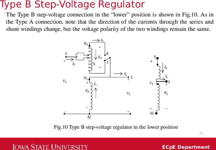
Type B Step-Voltage Regulator The Type B step-voltage connection in the “lower” position is shown in Fig.10. As in the Type A connection, note that the direction of the currents through the series and shunt windings change, but the voltage polarity of the two windings remain the same. Fig.10 Type B step-voltage regulator in the lower position 47 ECpE Department

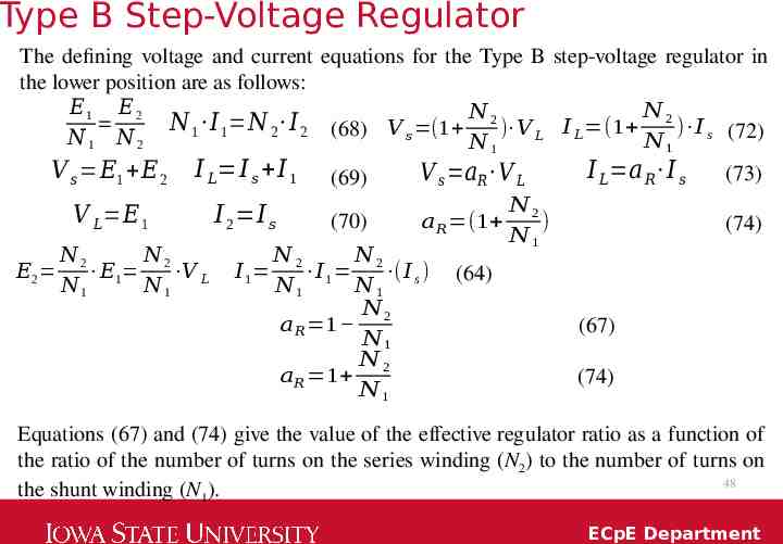
Type B Step-Voltage Regulator The defining voltage and current equations for the Type B step-voltage regulator in the lower position are as follows: 𝐸1 𝐸 2 𝑁 𝑁 1 𝐼 1 𝑁 2 𝐼 2 (68) 𝑉 𝑠 (1 𝑁 2 ) 𝑉 𝐿 𝐼 𝐿 (1 2 ) 𝐼 s (72) 𝑁1 𝑁2 𝑁1 𝑁1 𝑉 𝑠 𝐸1 𝐸 2 𝐼 𝐿 𝐼 𝑠 𝐼 1 (69) 𝐼 𝐿 𝑎 𝑅 𝐼 𝑠 𝑉 𝑠 𝑎𝑅 𝑉 𝐿 (73) 𝑁2 𝑉 𝐿 𝐸 1 𝐼 2 𝐼 𝑠 𝑎 𝑅 (1 ) (70) (74) 𝑁1 𝑁2 𝑁2 𝑁2 𝑁2 𝐸2 𝐸1 𝑉 𝐿 𝐼 1 𝐼1 ( 𝐼 s ) (64) 𝑁1 𝑁1 𝑁1 𝑁1 𝑁2 𝑎 𝑅 1 (67) 𝑁1 𝑁2 𝑎 𝑅 1 (74) 𝑁1 Equations (67) and (74) give the value of the effective regulator ratio as a function of the ratio of the number of turns on the series winding (N2) to the number of turns on 48 the shunt winding (N1). ECpE Department

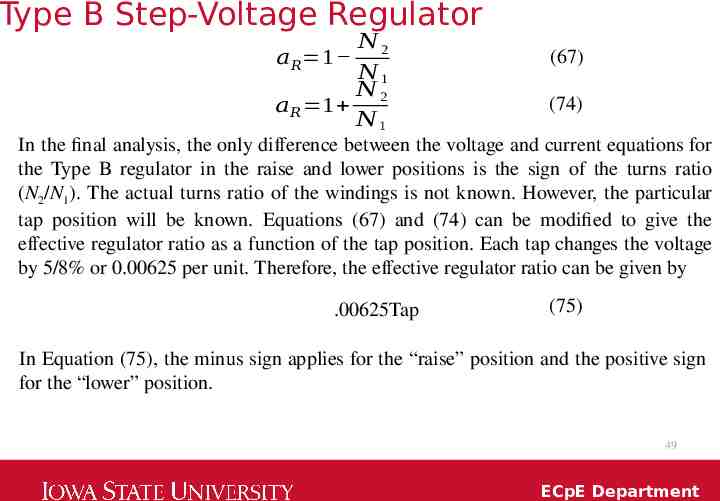
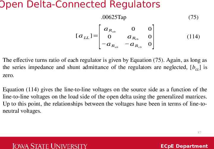
Type B Step-Voltage Regulator 𝑁2 𝑎 𝑅 1 𝑁1 𝑁2 𝑎 𝑅 1 𝑁1 (67) (74) In the final analysis, the only difference between the voltage and current equations for the Type B regulator in the raise and lower positions is the sign of the turns ratio (N2/N1). The actual turns ratio of the windings is not known. However, the particular tap position will be known. Equations (67) and (74) can be modified to give the effective regulator ratio as a function of the tap position. Each tap changes the voltage by 5/8% or 0.00625 per unit. Therefore, the effective regulator ratio can be given by .00625Tap (75) In Equation (75), the minus sign applies for the “raise” position and the positive sign for the “lower” position. 49 ECpE Department

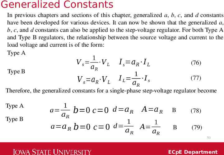
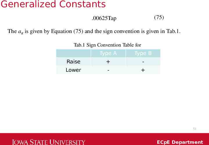
Generalized Constants In previous chapters and sections of this chapter, generalized a, b, c, and d constants have been developed for various devices. It can now be shown that the generalized a, b, c, and d constants can also be applied to the step-voltage regulator. For both Type A and Type B regulators, the relationship between the source voltage and current to the load voltage and current is of the form: Type A 1 𝑉 𝑠 𝑉 𝐿 𝑎𝑅 Type B 𝑉 𝑠 𝑎 𝑅 𝑉 𝐿 𝐼 s 𝑎 𝑅 𝐼 𝐿 (76) 1 𝐼 𝐿 𝐼 𝑠 𝑎𝑅 (77) Therefore, the generalized constants for a single-phase step-voltage regulator become Type A Type B a 1 𝑎𝑅 𝑏 0 c 0 d 𝑎 𝑅 𝐴 𝑎 𝑅 1 a 𝑎 𝑅 𝑏 0 c 0 d 𝑎 𝑅 1 𝐴 𝑎𝑅 B (78) B (79) 50 ECpE Department

Generalized Constants (75) .00625Tap The aR is given by Equation (75) and the sign convention is given in Tab.1. Tab.1 Sign Convention Table for Type A Type B Raise - Lower - 51 ECpE Department

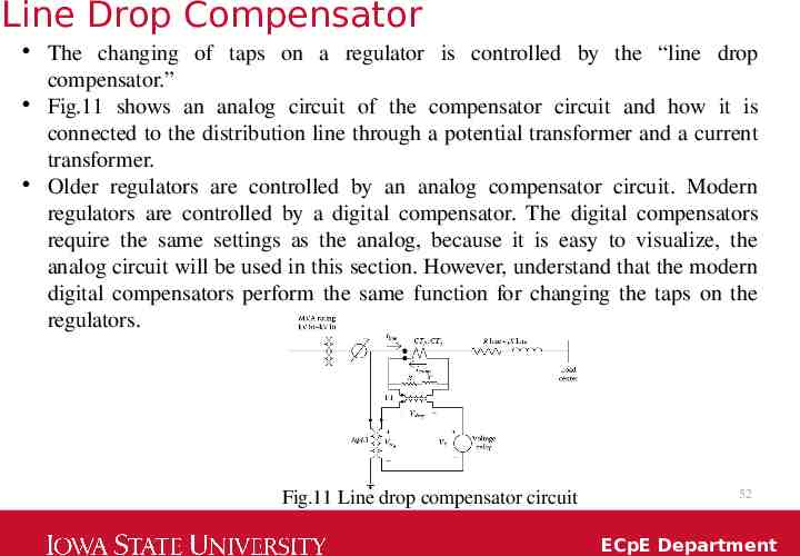
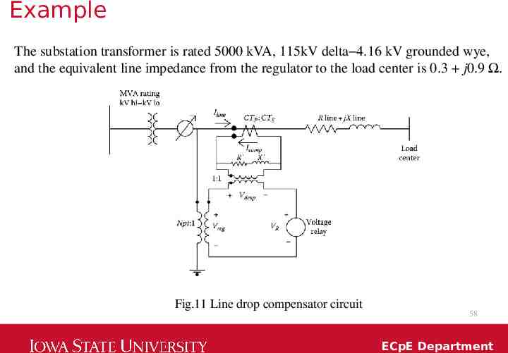
Line Drop Compensator The changing of taps on a regulator is controlled by the “line drop compensator.” Fig.11 shows an analog circuit of the compensator circuit and how it is connected to the distribution line through a potential transformer and a current transformer. Older regulators are controlled by an analog compensator circuit. Modern regulators are controlled by a digital compensator. The digital compensators require the same settings as the analog, because it is easy to visualize, the analog circuit will be used in this section. However, understand that the modern digital compensators perform the same function for changing the taps on the regulators. Fig.11 Line drop compensator circuit 52 ECpE Department

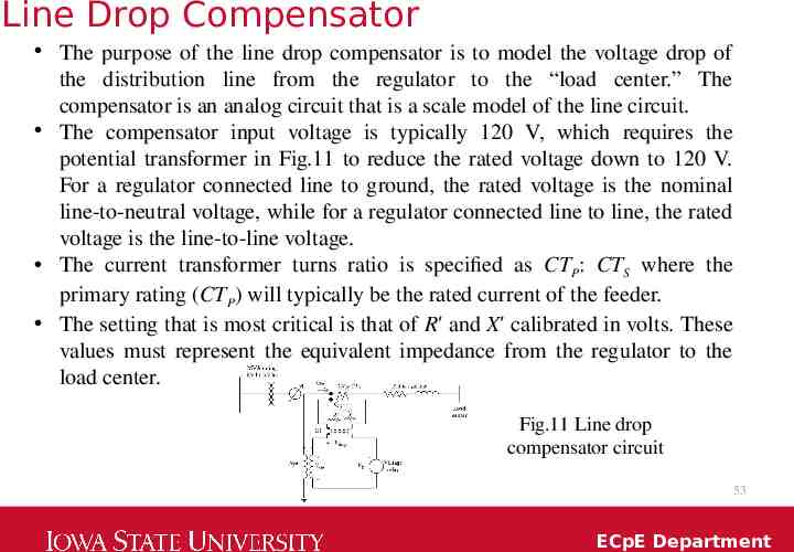
Line Drop Compensator The purpose of the line drop compensator is to model the voltage drop of the distribution line from the regulator to the “load center.” The compensator is an analog circuit that is a scale model of the line circuit. The compensator input voltage is typically 120 V, which requires the potential transformer in Fig.11 to reduce the rated voltage down to 120 V. For a regulator connected line to ground, the rated voltage is the nominal line-to-neutral voltage, while for a regulator connected line to line, the rated voltage is the line-to-line voltage. The current transformer turns ratio is specified as CTP: CTS where the primary rating (CTP) will typically be the rated current of the feeder. The setting that is most critical is that of R′ and X′ calibrated in volts. These values must represent the equivalent impedance from the regulator to the load center. Fig.11 Line drop compensator circuit 53 ECpE Department

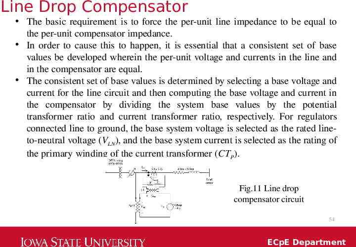
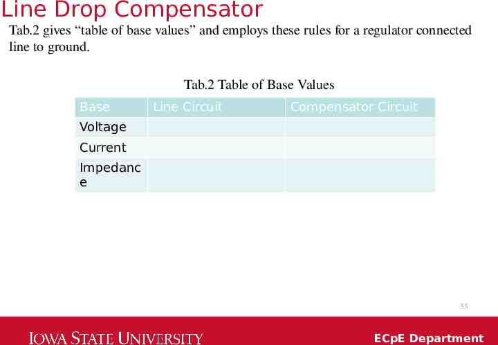
Line Drop Compensator The basic requirement is to force the per-unit line impedance to be equal to the per-unit compensator impedance. In order to cause this to happen, it is essential that a consistent set of base values be developed wherein the per-unit voltage and currents in the line and in the compensator are equal. The consistent set of base values is determined by selecting a base voltage and current for the line circuit and then computing the base voltage and current in the compensator by dividing the system base values by the potential transformer ratio and current transformer ratio, respectively. For regulators connected line to ground, the base system voltage is selected as the rated lineto-neutral voltage (VLN), and the base system current is selected as the rating of the primary winding of the current transformer (CTP). Fig.11 Line drop compensator circuit 54 ECpE Department

Line Drop Compensator Tab.2 gives “table of base values” and employs these rules for a regulator connected line to ground. Tab.2 Table of Base Values Base Line Circuit Compensator Circuit Voltage Current Impedanc e 55 ECpE Department

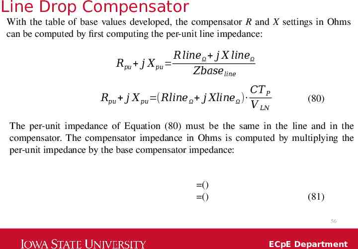
Line Drop Compensator With the table of base values developed, the compensator R and X settings in Ohms can be computed by first computing the per-unit line impedance: 𝑅 𝑙𝑖𝑛𝑒 Ω 𝑗 𝑋 𝑙𝑖𝑛𝑒Ω 𝑅𝑝𝑢 𝑗 𝑋 𝑝𝑢 𝑍𝑏𝑎𝑠𝑒 𝑙𝑖𝑛𝑒 𝐶𝑇 𝑃 𝑅𝑝𝑢 𝑗 𝑋 𝑝𝑢 (𝑅𝑙𝑖𝑛𝑒 Ω 𝑗 𝑋𝑙𝑖𝑛𝑒 Ω ) 𝑉 𝐿𝑁 (80) The per-unit impedance of Equation (80) must be the same in the line and in the compensator. The compensator impedance in Ohms is computed by multiplying the per-unit impedance by the base compensator impedance: () () (81) 56 ECpE Department

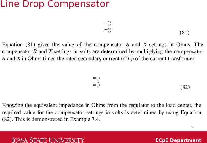
Line Drop Compensator () () (81) Equation (81) gives the value of the compensator R and X settings in Ohms. The compensator R and X settings in volts are determined by multiplying the compensator R and X in Ohms times the rated secondary current (CTS) of the current transformer: () () (82) Knowing the equivalent impedance in Ohms from the regulator to the load center, the required value for the compensator settings in volts is determined by using Equation (82). This is demonstrated in Example 7.4. 57 ECpE Department

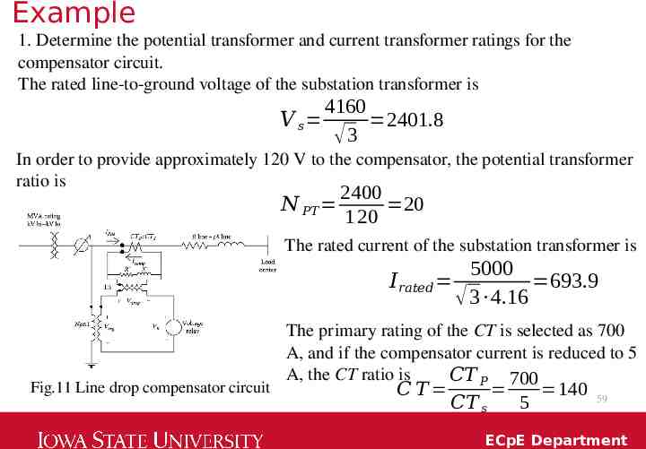
Example The substation transformer is rated 5000 kVA, 115kV delta 4.16 kV grounded wye, and the equivalent line impedance from the regulator to the load center is 0.3 j0.9 Ω. Fig.11 Line drop compensator circuit 58 ECpE Department

Example 1. Determine the potential transformer and current transformer ratings for the compensator circuit. The rated line-to-ground voltage of the substation transformer is 4160 𝑉 𝑠 2401.8 3 In order to provide approximately 120 V to the compensator, the potential transformer ratio is 𝑁 𝑃𝑇 2400 20 1 20 The rated current of the substation transformer is 5000 𝐼 𝑟𝑎𝑡𝑒𝑑 693.9 3 4.16 Fig.11 Line drop compensator circuit The primary rating of the CT is selected as 700 A, and if the compensator current is reduced to 5 A, the CT ratio is 𝐶𝑇 𝑃 700 𝐶𝑇 𝐶𝑇 𝑠 5 140 59 ECpE Department

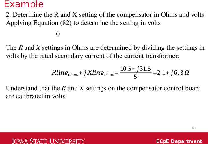
Example 2. Determine the R and X setting of the compensator in Ohms and volts Applying Equation (82) to determine the setting in volts () The R and X settings in Ohms are determined by dividing the settings in volts by the rated secondary current of the current transformer: 𝑅𝑙𝑖𝑛𝑒𝑜h𝑚𝑠 𝑗 𝑋𝑙𝑖𝑛𝑒 𝑜h𝑚𝑠 10.5 𝑗 31.5 2.1 𝑗 6 . 3 Ω 5 Understand that the R and X settings on the compensator control board are calibrated in volts. 60 ECpE Department

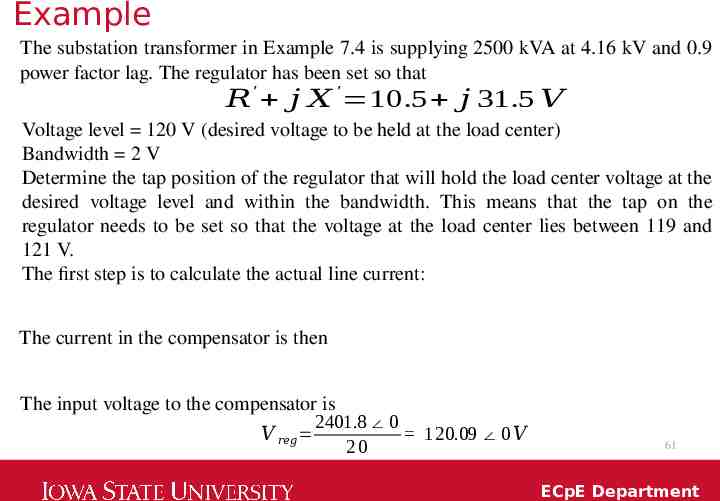
Example The substation transformer in Example 7.4 is supplying 2500 kVA at 4.16 kV and 0.9 power factor lag. The regulator has been set so that 𝑅′ 𝑗 𝑋 ′ 10.5 𝑗 31.5 𝑉 Voltage level 120 V (desired voltage to be held at the load center) Bandwidth 2 V Determine the tap position of the regulator that will hold the load center voltage at the desired voltage level and within the bandwidth. This means that the tap on the regulator needs to be set so that the voltage at the load center lies between 119 and 121 V. The first step is to calculate the actual line current: The current in the compensator is then The input voltage to the compensator is 2401.8 0 𝑉 𝑟𝑒𝑔 1 20.09 0 𝑉 20 61 ECpE Department

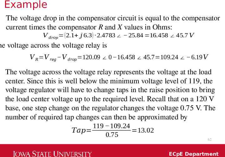
Example The voltage drop in the compensator circuit is equal to the compensator current times the compensator R and X values in Ohms: 𝑉 𝑑𝑟𝑜𝑝 ( 2.1 𝑗 6.3 ) 2.4783 25.84 16.458 45.7 𝑉 he voltage across the voltage relay is 𝑉 𝑅 𝑉 𝑟𝑒𝑔 𝑉 𝑑𝑟𝑜𝑝 120.09 0 16.458 45.7 109.24 6.19 𝑉 The voltage across the voltage relay represents the voltage at the load center. Since this is well below the minimum voltage level of 119, the voltage regulator will have to change taps in the raise position to bring the load center voltage up to the required level. Recall that on a 120 V base, one step change on the regulator changes the voltage 0.75 V. The number of required tap changes can then be approximated by 𝑇𝑎𝑝 119 109.24 13.02 0.75 62 ECpE Department

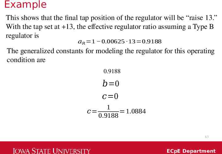
Example This shows that the final tap position of the regulator will be “raise 13.” With the tap set at 13, the effective regulator ratio assuming a Type B regulator is 𝑎 𝑅 1 0.00625 13 0.9188 The generalized constants for modeling the regulator for this operating condition are 0.9188 𝑏 0 𝑐 0 1 𝑐 1.0884 0.9188 63 ECpE Department

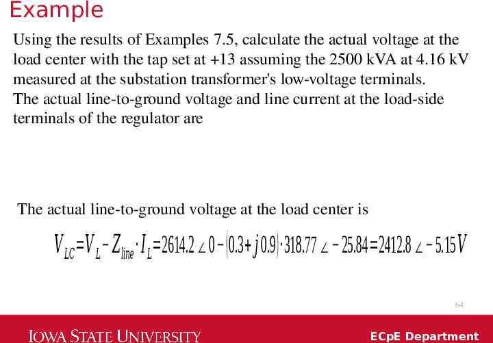
Example Using the results of Examples 7.5, calculate the actual voltage at the load center with the tap set at 13 assuming the 2500 kVA at 4.16 kV measured at the substation transformer's low-voltage terminals. The actual line-to-ground voltage and line current at the load-side terminals of the regulator are The actual line-to-ground voltage at the load center is 𝑉 𝐿𝐶 𝑉 𝐿 𝑍𝑙𝑖𝑛𝑒 𝐼 𝐿 2614.2 0 ( 0.3 𝑗0.9 ) 318.77 25.84 2412.8 5.15𝑉 64 ECpE Department

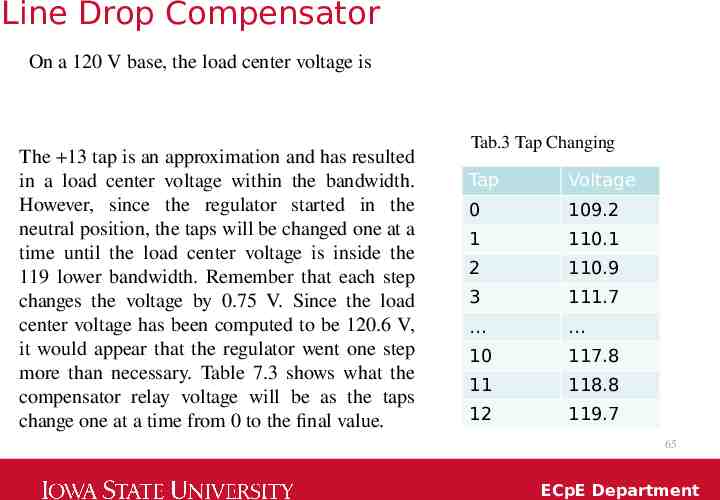
Line Drop Compensator On a 120 V base, the load center voltage is The 13 tap is an approximation and has resulted in a load center voltage within the bandwidth. However, since the regulator started in the neutral position, the taps will be changed one at a time until the load center voltage is inside the 119 lower bandwidth. Remember that each step changes the voltage by 0.75 V. Since the load center voltage has been computed to be 120.6 V, it would appear that the regulator went one step more than necessary. Table 7.3 shows what the compensator relay voltage will be as the taps change one at a time from 0 to the final value. Tab.3 Tap Changing Tap Voltage 0 109.2 1 110.1 2 110.9 3 111.7 10 117.8 11 118.8 12 119.7 65 ECpE Department

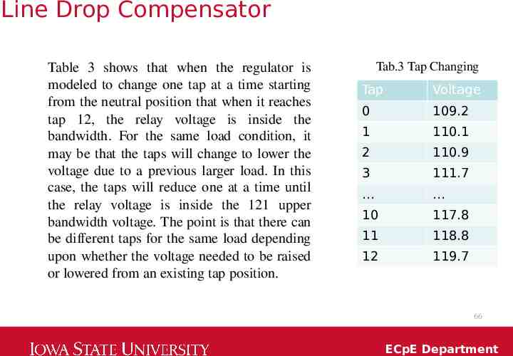
Line Drop Compensator Table 3 shows that when the regulator is modeled to change one tap at a time starting from the neutral position that when it reaches tap 12, the relay voltage is inside the bandwidth. For the same load condition, it may be that the taps will change to lower the voltage due to a previous larger load. In this case, the taps will reduce one at a time until the relay voltage is inside the 121 upper bandwidth voltage. The point is that there can be different taps for the same load depending upon whether the voltage needed to be raised or lowered from an existing tap position. Tab.3 Tap Changing Tap Voltage 0 109.2 1 110.1 2 110.9 3 111.7 10 117.8 11 118.8 12 119.7 66 ECpE Department

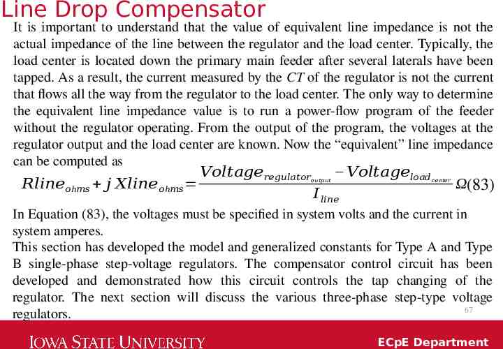
Line Drop Compensator It is important to understand that the value of equivalent line impedance is not the actual impedance of the line between the regulator and the load center. Typically, the load center is located down the primary main feeder after several laterals have been tapped. As a result, the current measured by the CT of the regulator is not the current that flows all the way from the regulator to the load center. The only way to determine the equivalent line impedance value is to run a power-flow program of the feeder without the regulator operating. From the output of the program, the voltages at the regulator output and the load center are known. Now the “equivalent” line impedance can be computed as 𝑅𝑙𝑖𝑛𝑒𝑜h𝑚𝑠 𝑗 𝑋𝑙𝑖𝑛𝑒 𝑜h𝑚𝑠 𝑉𝑜𝑙𝑡𝑎𝑔𝑒𝑟𝑒𝑔𝑢𝑙𝑎𝑡𝑜𝑟 𝑜𝑢𝑡𝑝𝑢𝑡 𝑉𝑜𝑙𝑡𝑎𝑔𝑒𝑙𝑜𝑎𝑑 𝐼 𝑙𝑖𝑛𝑒 𝑐𝑒𝑛𝑡𝑒𝑟 Ω(83) In Equation (83), the voltages must be specified in system volts and the current in system amperes. This section has developed the model and generalized constants for Type A and Type B single-phase step-voltage regulators. The compensator control circuit has been developed and demonstrated how this circuit controls the tap changing of the regulator. The next section will discuss the various three-phase step-type voltage 67 regulators. ECpE Department

Three-Phase Step-Voltage Regulator Three single-phase step-voltage regulators can be connected externally to form a three-phase regulator. When three single-phase regulators are connected together, each regulator has its own compensator circuit, and, therefore, the taps on each regulator are changed separately. Typical connections for single-phase stepregulators are 1. Single phase 2. Three regulators connected in grounded wye 3. Three regulators connected in closed delta 4. Two regulators connected in open delta 5. Two regulators connected in “open wye” (sometimes referred to as “V” phase) 68 ECpE Department

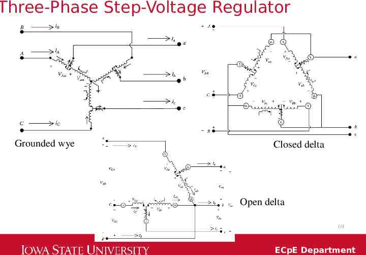
Three-Phase Step-Voltage Regulator Grounded wye Closed delta Open delta 69 ECpE Department

Three-Phase Step-Voltage Regulator A three-phase regulator has the connections between the single-phase windings internal to the regulator housing. The three-phase regulator is “gang” operated so that the taps on all windings change the same, and, as a result, only one compensator circuit is required. For this case, it is up to the engineer to determine which phase current and voltage will be sampled by the compensator circuit. Three-phase regulators will only be connected in a three-phase wye or closed delta. Many times the substation transformer will have LTC windings on the secondary. The LTC will be controlled in the same way as a gang-operated three-phase regulator. In the regulator models to be developed in the next sections, the phasing on the source side of the regulator will use capital letters A, B, and C. The load-side phasing will use lower case letters a, b, and c. 70 ECpE Department

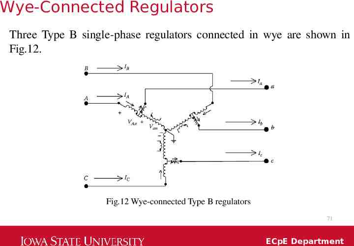
Wye-Connected Regulators Three Type B single-phase regulators connected in wye are shown in Fig.12. Fig.12 Wye-connected Type B regulators 71 ECpE Department

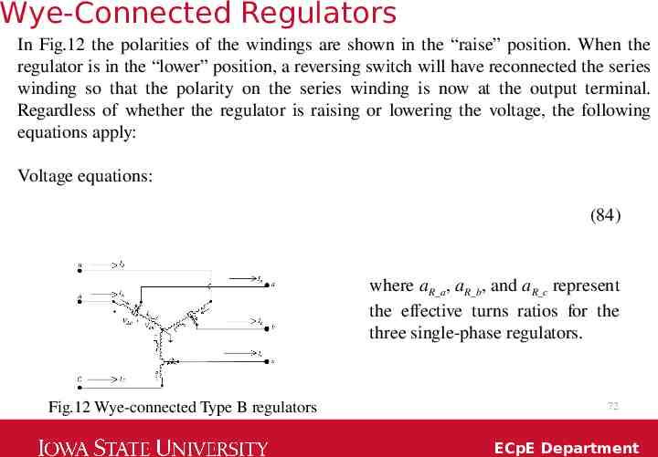
Wye-Connected Regulators In Fig.12 the polarities of the windings are shown in the “raise” position. When the regulator is in the “lower” position, a reversing switch will have reconnected the series winding so that the polarity on the series winding is now at the output terminal. Regardless of whether the regulator is raising or lowering the voltage, the following equations apply: Voltage equations: (84) where aR a, aR b, and aR c represent the effective turns ratios for the three single-phase regulators. Fig.12 Wye-connected Type B regulators 72 ECpE Department

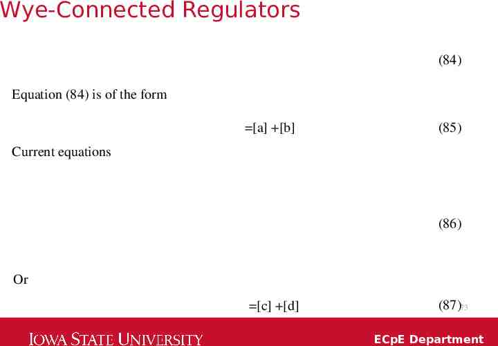
Wye-Connected Regulators (84) Equation (84) is of the form [a] [b] (85) Current equations (86) Or [c] [d] (87)73 ECpE Department

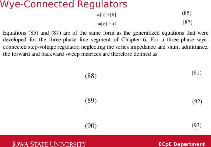
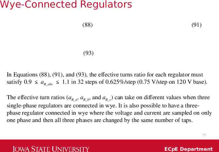
Wye-Connected Regulators [a] [b] (85) [c] [d] (87) Equations (85) and (87) are of the same form as the generalized equations that were developed for the three-phase line segment of Chapter 6. For a three-phase wyeconnected step-voltage regulator, neglecting the series impedance and shunt admittance, the forward and backward sweep matrices are therefore defined as (88) (91) (89) (92) (90) (93) 74 ECpE Department

Wye-Connected Regulators (88) (91) (93) In Equations (88), (91), and (93), the effective turns ratio for each regulator must satisfy 0.9 aR abc 1.1 in 32 steps of 0.625%/step (0.75 V/step on 120 V base). The effective turn ratios (aR a, aR b, and aR c) can take on different values when three single-phase regulators are connected in wye. It is also possible to have a threephase regulator connected in wye where the voltage and current are sampled on only one phase and then all three phases are changed by the same number of taps. 75 ECpE Department

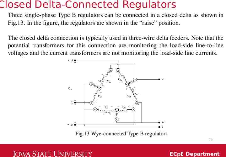
Closed Delta-Connected Regulators Three single-phase Type B regulators can be connected in a closed delta as shown in Fig.13. In the figure, the regulators are shown in the “raise” position. The closed delta connection is typically used in three-wire delta feeders. Note that the potential transformers for this connection are monitoring the load-side line-to-line voltages and the current transformers are not monitoring the load-side line currents. Fig.13 Wye-connected Type B regulators 76 ECpE Department

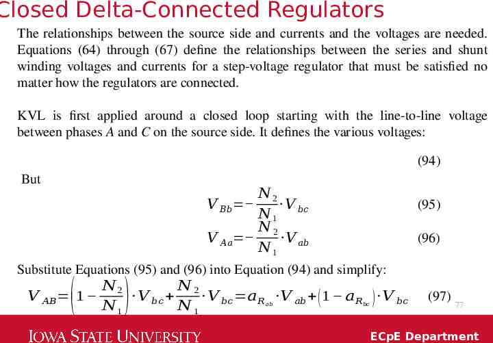
Closed Delta-Connected Regulators The relationships between the source side and currents and the voltages are needed. Equations (64) through (67) define the relationships between the series and shunt winding voltages and currents for a step-voltage regulator that must be satisfied no matter how the regulators are connected. KVL is first applied around a closed loop starting with the line-to-line voltage between phases A and C on the source side. It defines the various voltages: (94) But 𝑁2 𝑉 𝐵𝑏 𝑉 𝑁 1 𝑏𝑐 𝑁2 𝑉 𝐴𝑎 𝑉 𝑎𝑏 𝑁1 (95) (96) Substitute Equations (95) and (96) into Equation (94) and simplify: 𝑁 𝑁 𝑉 𝐴𝐵 1 2 𝑉 𝑏𝑐 2 𝑉 𝑏𝑐 𝑎 𝑅 𝑉 𝑎𝑏 ( 1 𝑎 𝑅 ) 𝑉 𝑏𝑐 𝑁1 𝑁1 ( ) 𝑎𝑏 𝑏𝑐 (97) 77 ECpE Department

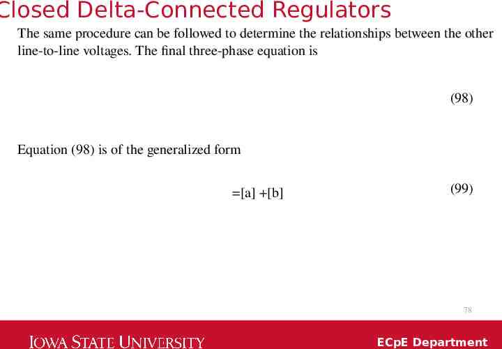
Closed Delta-Connected Regulators The same procedure can be followed to determine the relationships between the other line-to-line voltages. The final three-phase equation is (98) Equation (98) is of the generalized form [a] [b] (99) 78 ECpE Department

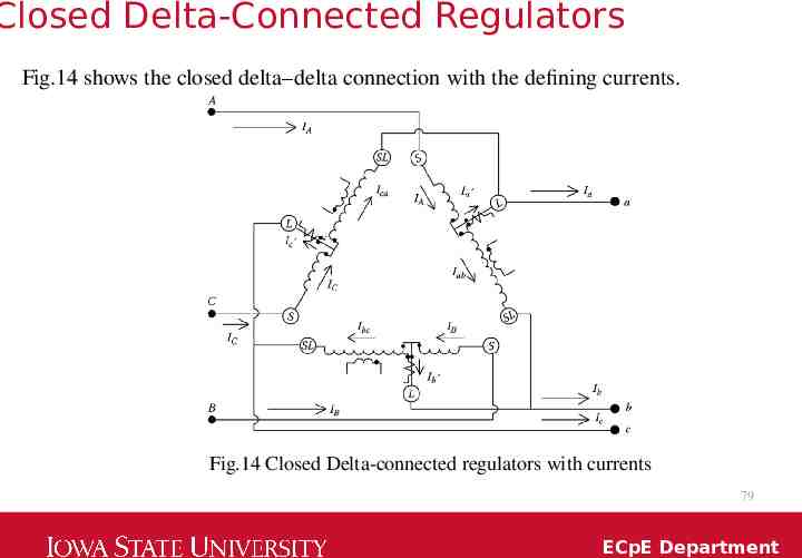
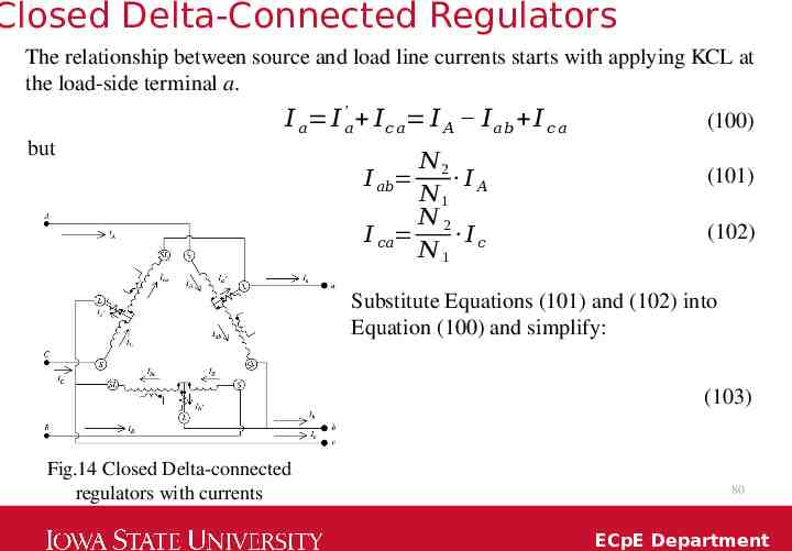
Closed Delta-Connected Regulators Fig.14 shows the closed delta–delta connection with the defining currents. Fig.14 Closed Delta-connected regulators with currents 79 ECpE Department

Closed Delta-Connected Regulators The relationship between source and load line currents starts with applying KCL at the load-side terminal a. 𝐼 𝑎 𝐼 ′𝑎 𝐼 𝑐 𝑎 𝐼 𝐴 𝐼 𝑎 𝑏 𝐼 𝑐 𝑎 but 𝑁2 𝐼 𝑎𝑏 𝐼 𝑁1 𝐴 𝑁2 𝐼 𝑐𝑎 𝐼𝑐 𝑁1 (100) (101) (102) Substitute Equations (101) and (102) into Equation (100) and simplify: (103) Fig.14 Closed Delta-connected regulators with currents 80 ECpE Department

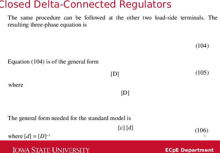
Closed Delta-Connected Regulators The same procedure can be followed at the other two load-side terminals. The resulting three-phase equation is (104) Equation (104) is of the general form (105) [D] where [D] The general form needed for the standard model is [c] [d] where [d] [D] 1 (106) 81 ECpE Department

Closed Delta-Connected Regulators As with the wye-connected regulators, the matrices [b] and [c] are zero as long as the series impedance and shunt admittance of each regulator are neglected. The closed delta connection can be difficult to apply. Note that in both the voltage and current equations, a change of the tap position in one regulator will affect voltages and currents in two phases. As a result, increasing the tap in one regulator will affect the tap position of the second regulator. In most cases, the bandwidth setting for the closed delta connection will have to be wider than that for wye-connected regulators. 82 ECpE Department

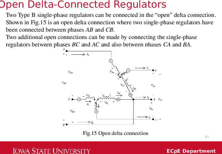
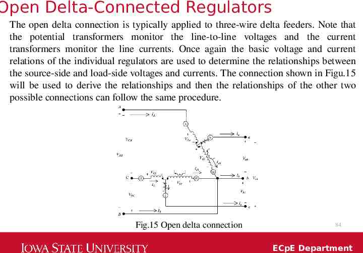
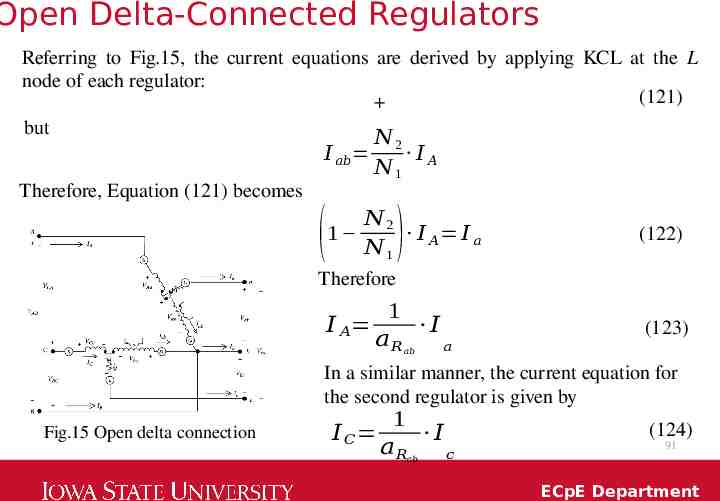
Open Delta-Connected Regulators Two Type B single-phase regulators can be connected in the “open” delta connection. Shown in Fig.15 is an open delta connection where two single-phase regulators have been connected between phases AB and CB. Two additional open connections can be made by connecting the single-phase regulators between phases BC and AC and also between phases CA and BA. Fig.15 Open delta connection 83 ECpE Department

Open Delta-Connected Regulators The open delta connection is typically applied to three-wire delta feeders. Note that the potential transformers monitor the line-to-line voltages and the current transformers monitor the line currents. Once again the basic voltage and current relations of the individual regulators are used to determine the relationships between the source-side and load-side voltages and currents. The connection shown in Figu.15 will be used to derive the relationships and then the relationships of the other two possible connections can follow the same procedure. Fig.15 Open delta connection 84 ECpE Department

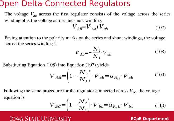
Open Delta-Connected Regulators The voltage VAB across the first regulator consists of the voltage across the series winding plus the voltage across the shunt winding: 𝑉 𝐴𝐵 𝑉 𝐴𝑎 𝑉 𝑎𝑏 (107) Paying attention to the polarity marks on the series and shunt windings, the voltage across the series winding is 𝑁2 𝑉 𝐴𝑏 𝑉 𝑁 1 𝑎𝑏 (108) Substituting Equation (108) into Equation (107) yields 𝑁2 𝑉 𝐴𝐵 1 𝑉 𝑎𝑏 𝑎 𝑅 𝑉 𝑎𝑏 𝑁1 ( ) 𝑎𝑏 (109) Following the same procedure for the regulator connected across VBC, the voltage equation is 𝑁2 𝑉 𝐵𝐶 1 𝑉 𝑏𝑐 𝑎 𝑅 𝑏 𝑉 𝑏𝑐 (110) 85 𝑁1 ( ) 𝑐 ECpE Department

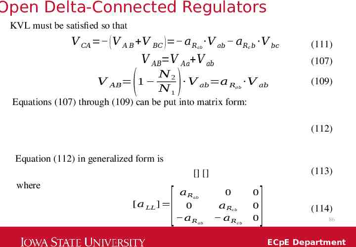
Open Delta-Connected Regulators KVL must be satisfied so that 𝑉 𝐶𝐴 ( 𝑉 𝐴 𝐵 𝑉 𝐵𝐶 ) 𝑎 𝑅 𝑉 𝑎𝑏 𝑎 𝑅 𝑏 𝑉 𝑏𝑐 (111) 𝑉 𝐴𝐵 𝑉 𝐴𝑎 𝑉 𝑎𝑏 (107) 𝑎𝑏 𝑐 𝑁2 𝑉 𝑎𝑏 𝑎 𝑅 𝑉 𝑎𝑏 𝑁1 Equations (107) through (109) can be put into matrix form: ( ) 𝑉 𝐴𝐵 1 𝑎𝑏 (109) (112) Equation (112) in generalized form is (113) [] [] where 𝑎𝑅 [ 𝑎 𝐿𝐿 ] 0 𝑎𝑅 [ 𝑎𝑏 0 𝑎𝑅 𝑎𝑅 𝑐𝑏 𝑎𝑏 𝑐𝑏 0 0 0 ] (114) 86 ECpE Department

Open Delta-Connected Regulators .00625Tap 𝑎𝑅 [ 𝑎 𝐿𝐿 ] 0 𝑎𝑅 [ 𝑎𝑏 (75) 0 𝑎𝑅 𝑎𝑅 𝑐𝑏 𝑎𝑏 𝑐𝑏 0 0 0 ] (114) The effective turns ratio of each regulator is given by Equation (75). Again, as long as the series impedance and shunt admittance of the regulators are neglected, [bLL] is zero. Equation (114) gives the line-to-line voltages on the source side as a function of the line-to-line voltages on the load side of the open delta using the generalized matrices. Up to this point, the relationships between the voltages have been in terms of line-toneutral voltages. 87 ECpE Department

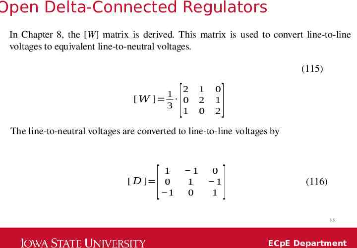
Open Delta-Connected Regulators In Chapter 8, the [W] matrix is derived. This matrix is used to convert line-to-line voltages to equivalent line-to-neutral voltages. (115) 2 1 [ 𝑊 ] 0 3 1 [ 1 2 0 0 1 2 ] The line-to-neutral voltages are converted to line-to-line voltages by 1 [ 𝐷 ] 0 1 [ 1 1 0 0 1 1 ] (116) 88 ECpE Department

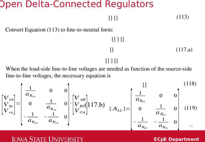
Open Delta-Connected Regulators (113) [] [] Convert Equation (113) to line-to-neutral form: [] ] [] [] (117.a) [] ] [] When the load-side line-to-line voltages are needed as function of the source-side line-to-line voltages, the necessary equation is (118) [] 𝑉 𝑎𝑏 𝑉 𝑏𝑐 𝑉 𝑐𝑎 [ ] [ 1 𝑎𝑅 0 0 𝑎𝑏 0 1 𝑎𝑅 1 𝑎𝑅 𝑐𝑏 1 𝑎𝑅 𝑎𝑏 𝑐𝑏 ] 𝑉 𝐴𝐵 0 𝑉 𝐵𝐶(117.b) 𝑉 𝐶𝐴 0 [ ] [ 𝐴 𝐿𝐿 ] [ 1 𝑎𝑅 0 0 𝑎𝑏 0 1 𝑎𝑅 1 𝑎𝑅 0 𝑐𝑏 1 𝑎𝑅 𝑎𝑏 𝑐𝑏 0 ] (119) 89 ECpE Department

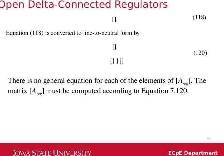
Open Delta-Connected Regulators [] (118) Equation (118) is converted to line-to-neutral form by [] (120) [] ] [] There is no general equation for each of the elements of [Areg]. The matrix [Areg] must be computed according to Equation 7.120. 90 ECpE Department

Open Delta-Connected Regulators Referring to Fig.15, the current equations are derived by applying KCL at the L node of each regulator: (121) but 𝑁 𝐼 𝑎𝑏 2 𝐼𝐴 𝑁1 Therefore, Equation (121) becomes 𝑁2 𝐼 𝐴 𝐼 𝑎 𝑁1 Therefore ( ) 1 𝐼 𝐴 1 𝐼 𝑎𝑅 𝑎 (122) (123) 𝑎𝑏 In a similar manner, the current equation for the second regulator is given by Fig.15 Open delta connection 𝐼 𝐶 1 𝐼 𝑎𝑅 𝑐 (124) 91 𝑐𝑏 ECpE Department

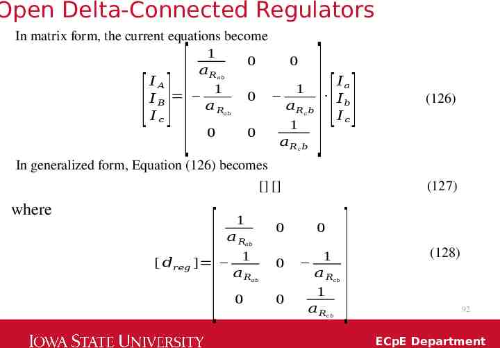
Open Delta-Connected Regulators In matrix form, the current equations become 𝐼𝐴 𝐼𝐵 𝐼𝑐 1 𝑎𝑅 1 𝑎𝑅 [] [ 0 0 𝑎𝑏 0 𝑎𝑏 1 𝑎𝑅 𝑏 1 𝑎𝑅 𝑏 𝑐 0 0 𝑐 ] 𝐼𝑎 𝐼𝑏 𝐼𝑐 [] In generalized form, Equation (126) becomes [] [] where 1 𝑎𝑅 [ 𝑑𝑟𝑒𝑔 ] 1 𝑎𝑅 [ 0 (127) 0 𝑎𝑏 0 𝑎𝑏 0 1 𝑎𝑅 1 𝑎𝑅 𝑐𝑏 0 (126) 𝑐𝑏 ] (128) 92 ECpE Department

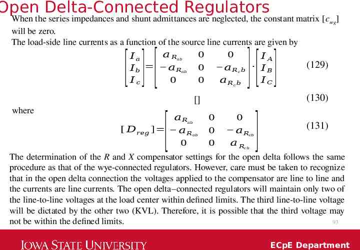
Open Delta-Connected Regulators When the series impedances and shunt admittances are neglected, the constant matrix [creg] will be zero. The load-side line currents as a function of the source line currents are given by 𝑎𝑅 0 0 𝐼𝑎 𝐼𝐴 (129) 0 𝑎𝑅 𝑏 𝐼 𝐵 𝐼 𝑏 𝑎𝑅 𝐼𝑐 0 0 𝑎𝑅 𝑏 𝐼𝐶 [ ][ 𝑎𝑏 𝑎𝑏 𝑐 𝑐 ][ ] (130) [] where 𝑎𝑅 0 0 (131) [ 𝐷𝑟𝑒𝑔 ] 𝑎 𝑅 0 𝑎𝑅 0 0 𝑎𝑅 The determination of the R and X compensator settings for the open delta follows the same procedure as that of the wye-connected regulators. However, care must be taken to recognize that in the open delta connection the voltages applied to the compensator are line to line and the currents are line currents. The open delta–connected regulators will maintain only two of the line-to-line voltages at the load center within defined limits. The third line-to-line voltage will be dictated by the other two (KVL). Therefore, it is possible that the third voltage may not be within the defined limits. 93 [ 𝑎𝑏 𝑎𝑏 𝑐𝑏 𝑐𝑏 ] ECpE Department

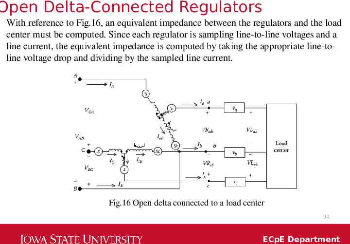
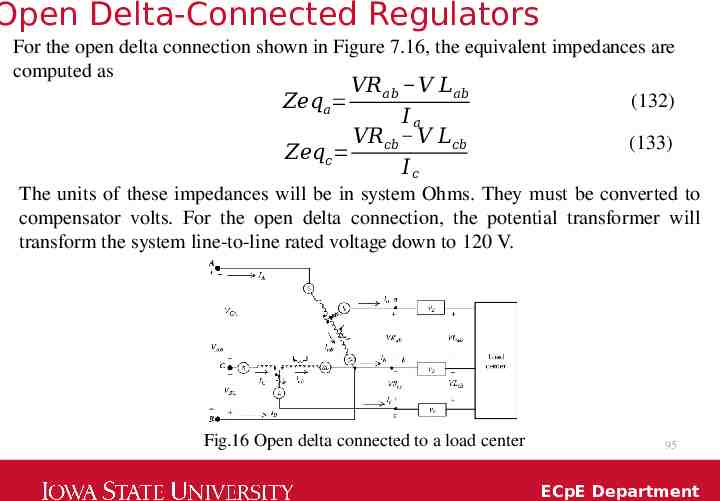
Open Delta-Connected Regulators With reference to Fig.16, an equivalent impedance between the regulators and the load center must be computed. Since each regulator is sampling line-to-line voltages and a line current, the equivalent impedance is computed by taking the appropriate line-toline voltage drop and dividing by the sampled line current. Fig.16 Open delta connected to a load center 94 ECpE Department

Open Delta-Connected Regulators For the open delta connection shown in Figure 7.16, the equivalent impedances are computed as 𝑉𝑅 𝑎 𝑏 𝑉 𝐿𝑎𝑏 𝑍𝑒𝑞𝑎 𝐼𝑎 𝑉𝑅𝑐𝑏 𝑉 𝐿𝑐𝑏 𝑍𝑒𝑞𝑐 𝐼𝑐 (132) (133) The units of these impedances will be in system Ohms. They must be converted to compensator volts. For the open delta connection, the potential transformer will transform the system line-to-line rated voltage down to 120 V. Fig.16 Open delta connected to a load center 95 ECpE Department

Thank You! 96 ECpE Department