CS 473-Algorithms I SINGLE-SOURCE SHORTEST PATHS CS473 LectureX 1
83 Slides953.50 KB
CS 473-Algorithms I SINGLE-SOURCE SHORTEST PATHS CS473 LectureX 1
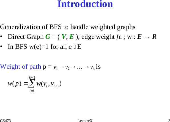
Introduction Generalization of BFS to handle weighted graphs Direct Graph G ( V, E ), edge weight fn ; w : E R In BFS w(e) 1 for all e E Weight of path p v1 v2 vk is k 1 w( p) w(vi , vi 1 ) i 1 CS473 LectureX 2
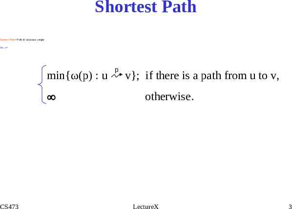
Shortest Path Shortest Path Path of minimum weight δ(u,v) min{ω(p) : u CS473 p v}; if there is a path from u to v, otherwise. LectureX 3
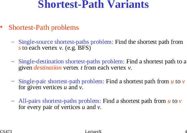
Shortest-Path Variants Shortest-Path problems – Single-source shortest-paths problem: Find the shortest path from s to each vertex v. (e.g. BFS) – Single-destination shortest-paths problem: Find a shortest path to a given destination vertex t from each vertex v. – Single-pair shortest-path problem: Find a shortest path from u to v for given vertices u and v. – All-pairs shortest-paths problem: Find a shortest path from u to v for every pair of vertices u and v. CS473 LectureX 4
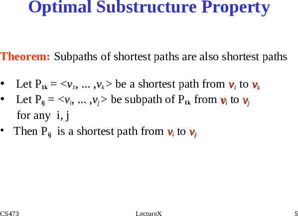
Optimal Substructure Property Theorem: Subpaths of shortest paths are also shortest paths Let P1k v1, . ,vk be a shortest path from v1 to vk Let Pij vi, . ,vj be subpath of P1k from vi to vj for any i, j Then Pij is a shortest path from vi to vj CS473 LectureX 5
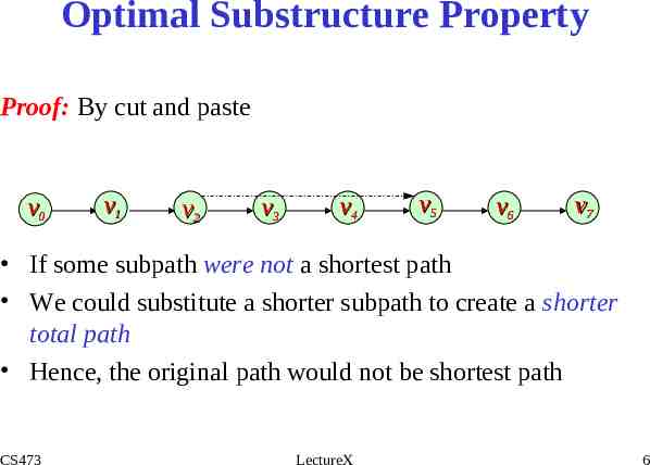
Optimal Substructure Property Proof: By cut and paste v0 v1 v2 v3 v4 v5 v6 v7 If some subpath were not a shortest path We could substitute a shorter subpath to create a shorter total path Hence, the original path would not be shortest path CS473 LectureX 6
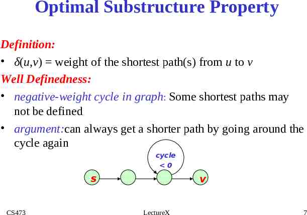
Optimal Substructure Property Definition: δ(u,v) weight of the shortest path(s) from u to v Well Definedness: negative-weight cycle in graph: Some shortest paths may not be defined argument:can always get a shorter path by going around the cycle again cycle 0 s CS473 v LectureX 7
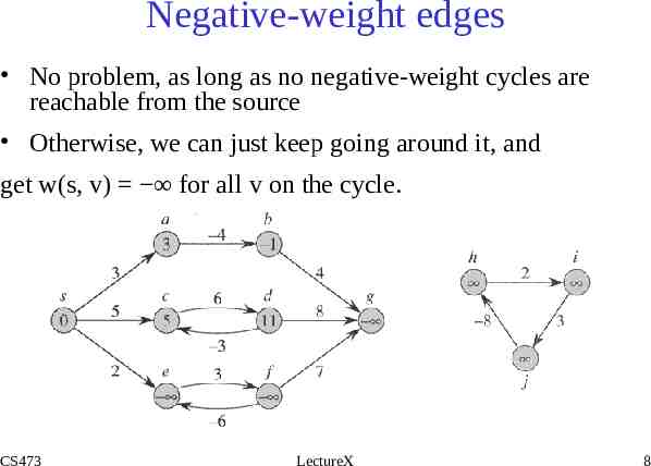
Negative-weight edges No problem, as long as no negative-weight cycles are reachable from the source Otherwise, we can just keep going around it, and get w(s, v) for all v on the cycle. CS473 LectureX 8
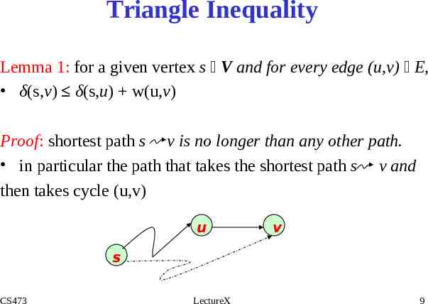
Triangle Inequality Lemma 1: for a given vertex s V and for every edge (u,v) E, δ(s,v) δ(s,u) w(u,v) Proof: shortest path s v is no longer than any other path. in particular the path that takes the shortest path s v and then takes cycle (u,v) u v s CS473 LectureX 9
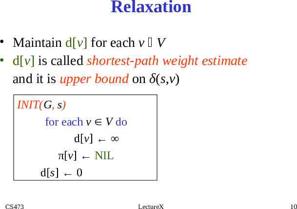
Relaxation Maintain d[v] for each v V d[v] is called shortest-path weight estimate and it is upper bound on δ(s,v) INIT(G, s) for each v V do d[v] π[v] NIL d[s] 0 CS473 LectureX 10
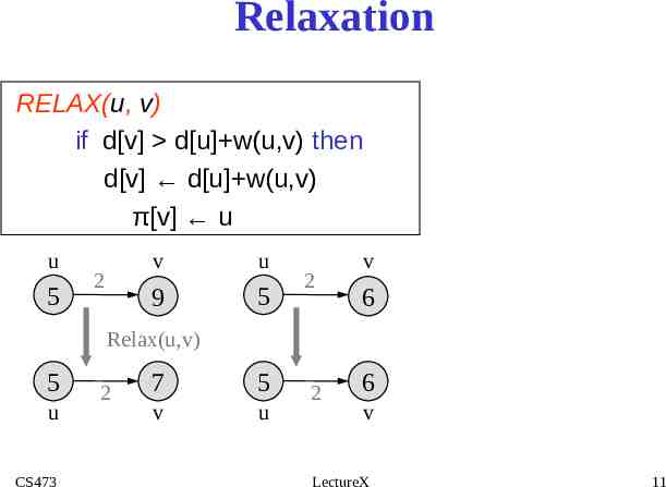
Relaxation RELAX(u, v) if d[v] d[u] w(u,v) then d[v] d[u] w(u,v) π[v] u u 2 v u 2 v Relax(u,v) u CS473 2 v u 2 v LectureX 11
Properties of Relaxation Algorithms differ in how many times they relax each edge, and the order in which they relax edges Question: How many times each edge is relaxed in BFS? Answer: Only once! CS473 LectureX 12
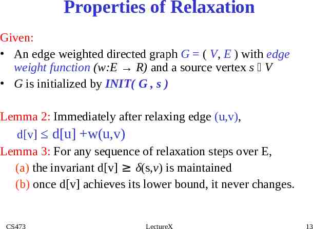
Properties of Relaxation Given: An edge weighted directed graph G ( V, E ) with edge weight function (w:E R) and a source vertex s V G is initialized by INIT( G , s ) Lemma 2: Immediately after relaxing edge (u,v), d[v] d[u] w(u,v) Lemma 3: For any sequence of relaxation steps over E, (a) the invariant d[v] δ(s,v) is maintained (b) once d[v] achieves its lower bound, it never changes. CS473 LectureX 13
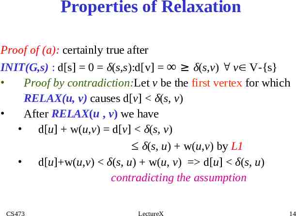
Properties of Relaxation Proof of (a): certainly true after INIT(G,s) : d[s] 0 δ(s,s):d[v] δ(s,v) v V-{s} Proof by contradiction:Let v be the first vertex for which RELAX(u, v) causes d[v] δ(s, v) After RELAX(u , v) we have d[u] w(u,v) d[v] δ(s, v) δ(s, u) w(u,v) by L1 d[u] w(u,v) δ(s, u) w(u, v) d[u] δ(s, u) contradicting the assumption CS473 LectureX 14
Properties of Relaxation Proof of (b): d[v] cannot decrease after achieving its lower bound; because d[v] δ(s,v) d[v] cannot increase since relaxations don’t increase d values. CS473 LectureX 15
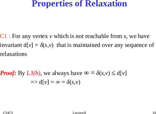
Properties of Relaxation C1 : For any vertex v which is not reachable from s, we have invariant d[v] δ(s,v) that is maintained over any sequence of relaxations Proof: By L3(b), we always have δ(s,v) d[v] d[v] δ(s,v) CS473 LectureX 16
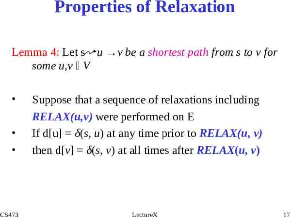
Properties of Relaxation Lemma 4: Let s u v be a shortest path from s to v for some u,v V CS473 Suppose that a sequence of relaxations including RELAX(u,v) were performed on E If d[u] δ(s, u) at any time prior to RELAX(u, v) then d[v] δ(s, v) at all times after RELAX(u, v) LectureX 17
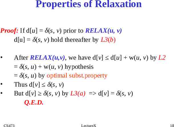
Properties of Relaxation Proof: If d[u] δ(s, v) prior to RELAX(u, v) d[u] δ(s, v) hold thereafter by L3(b) After RELAX(u,v), we have d[v] d[u] w(u, v) by L2 δ(s, u) w(u, v) hypothesis δ(s, u) by optimal subst.property Thus d[v] δ(s, v) But d[v] δ(s, v) by L3(a) d[v] δ(s, v) Q.E.D. CS473 LectureX 18
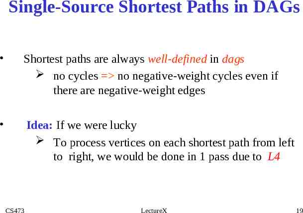
Single-Source Shortest Paths in DAGs Shortest paths are always well-defined in dags no cycles no negative-weight cycles even if there are negative-weight edges Idea: If we were lucky To process vertices on each shortest path from left to right, we would be done in 1 pass due to L4 CS473 LectureX 19
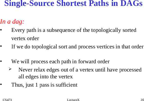
Single-Source Shortest Paths in DAGs In a dag: Every path is a subsequence of the topologically sorted vertex order If we do topological sort and process vertices in that order We will process each path in forward order Never relax edges out of a vertex until have processed all edges into the vertex Thus, just 1 pass is sufficient CS473 LectureX 20
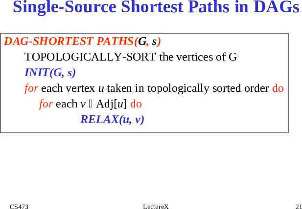
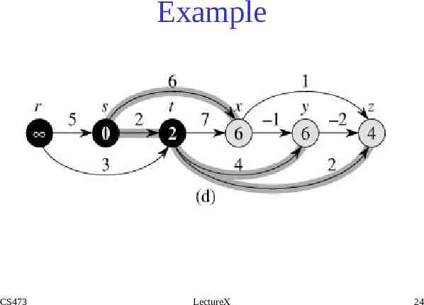
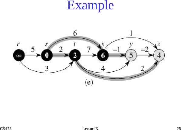
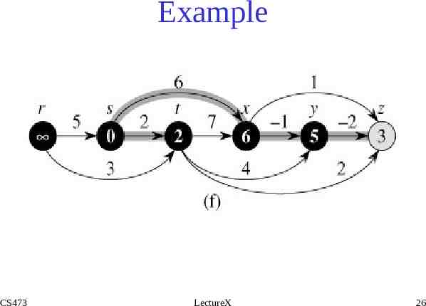
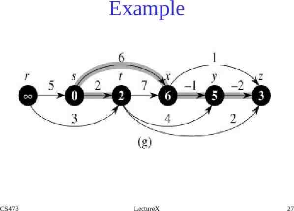
Single-Source Shortest Paths in DAGs DAG-SHORTEST PATHS(G, s) TOPOLOGICALLY-SORT the vertices of G INIT(G, s) for each vertex u taken in topologically sorted order do for each v Adj[u] do RELAX(u, v) CS473 LectureX 21
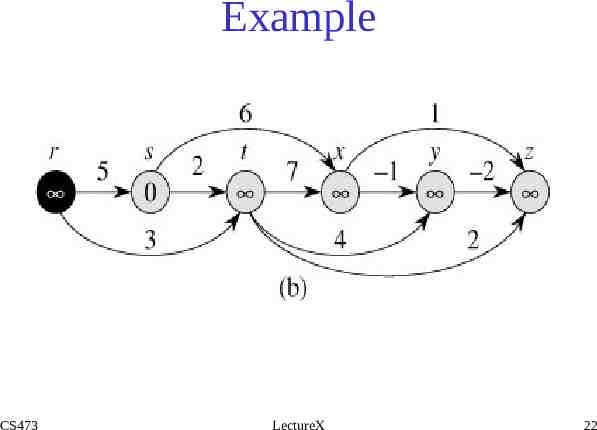
Example CS473 LectureX 22
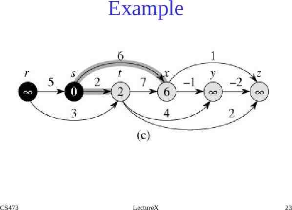
Example CS473 LectureX 23
Example CS473 LectureX 24
Example CS473 LectureX 25
Example CS473 LectureX 26
Example CS473 LectureX 27
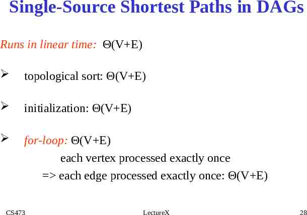
Single-Source Shortest Paths in DAGs Runs in linear time: Θ(V E) topological sort: Θ(V E) initialization: Θ(V E) for-loop: Θ(V E) each vertex processed exactly once each edge processed exactly once: Θ(V E) CS473 LectureX 28
Single-Source Shortest Paths in DAGs Thm: (Correctness of DAG-SHORTEST-PATHS): At termination of DAG-SHORTEST-PATHS procedure d[v] δ(s, v) for all v V CS473 LectureX 29
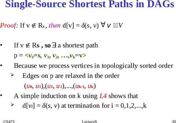
Single-Source Shortest Paths in DAGs v V E A Proof: If v Rs , then d[v] δ(s, v) If v Rs , so a shortest path p v0 s, v1, v2, ,vk v Because we process vertices in topologically sorted order Edges on p are relaxed in the order (u0, u1),(u1, u2),.,(uk-1, uk) A simple induction on k using L4 shows that d[vi] δ(s, v) at termination for i 0,1,2,.,k CS473 LectureX 30
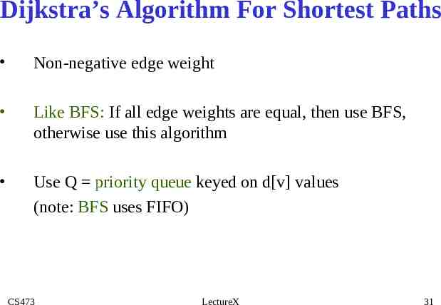
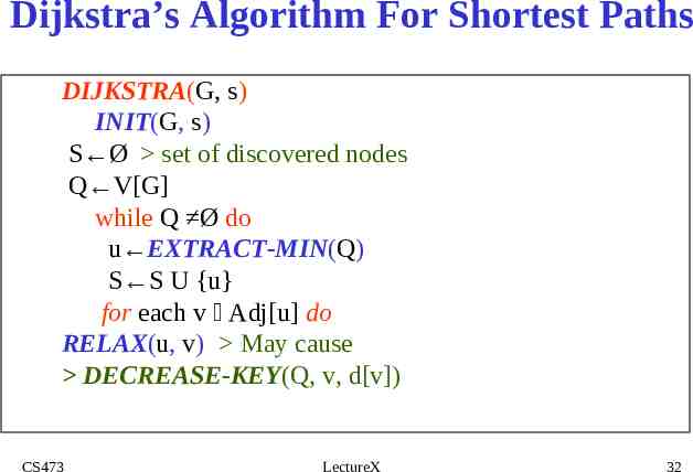
Dijkstra’s Algorithm For Shortest Paths Non-negative edge weight Like BFS: If all edge weights are equal, then use BFS, otherwise use this algorithm Use Q priority queue keyed on d[v] values (note: BFS uses FIFO) CS473 LectureX 31
Dijkstra’s Algorithm For Shortest Paths DIJKSTRA(G, s) INIT(G, s) S Ø set of discovered nodes Q V[G] while Q Ø do u EXTRACT-MIN(Q) S S U {u} for each v Adj[u] do RELAX(u, v) May cause DECREASE-KEY(Q, v, d[v]) CS473 LectureX 32
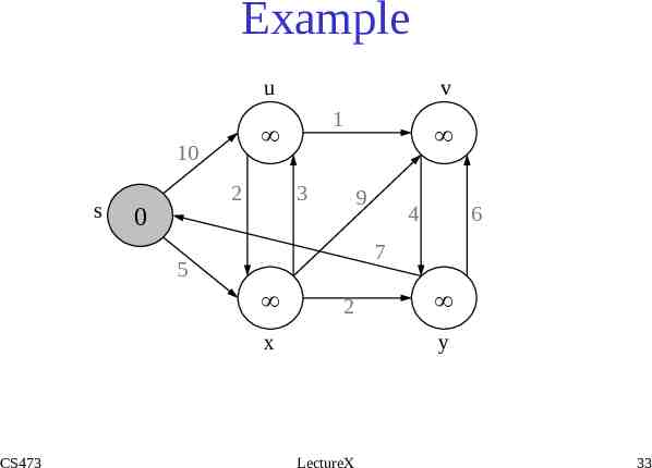
Example u 1 10 s v 2 3 9 4 6 7 5 2 x CS473 y LectureX 33
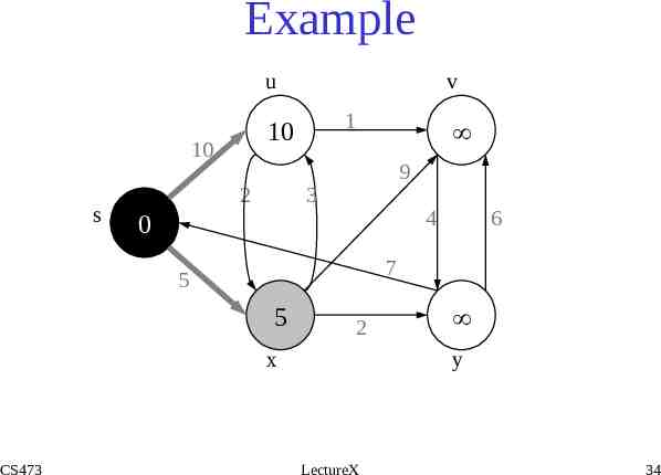
Example u 1 10 s v 2 9 3 4 7 5 2 x CS473 6 y LectureX 34
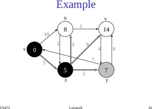
Example u 1 10 s v 2 9 3 6 7 5 2 x CS473 4 y LectureX 35
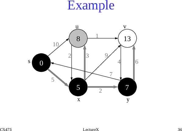
Example u 1 10 s v 2 9 3 6 7 5 2 x CS473 4 y LectureX 36
Example u 1 10 s v 2 3 9 4 6 7 5 2 x CS473 y LectureX 37
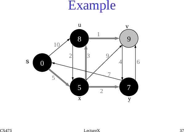
Example u 1 10 2 s v 9 3 4 7 5 2 x CS473 6 y LectureX 38
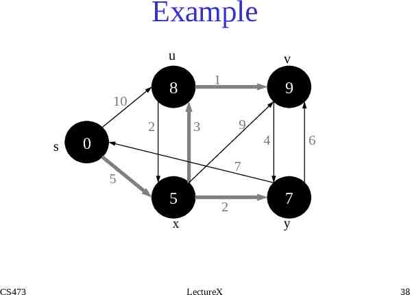
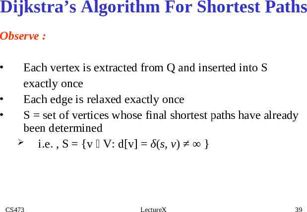
Dijkstra’s Algorithm For Shortest Paths Observe : Each vertex is extracted from Q and inserted into S exactly once Each edge is relaxed exactly once S set of vertices whose final shortest paths have already been determined i.e. , S {v V: d[v] δ(s, v) } CS473 LectureX 39
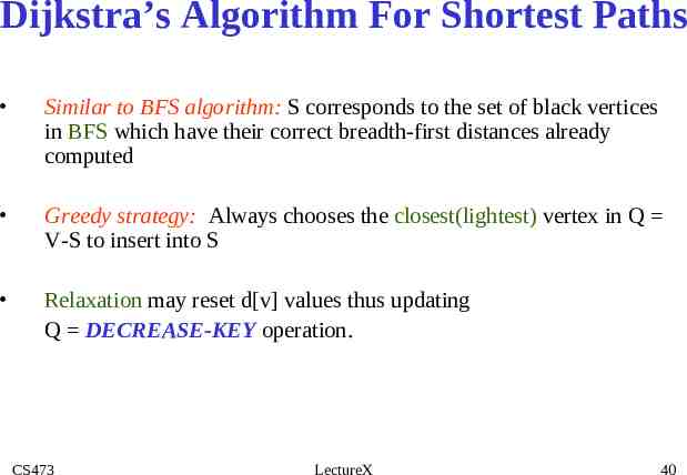
Dijkstra’s Algorithm For Shortest Paths Similar to BFS algorithm: S corresponds to the set of black vertices in BFS which have their correct breadth-first distances already computed Greedy strategy: Always chooses the closest(lightest) vertex in Q V-S to insert into S Relaxation may reset d[v] values thus updating Q DECREASE-KEY operation. CS473 LectureX 40
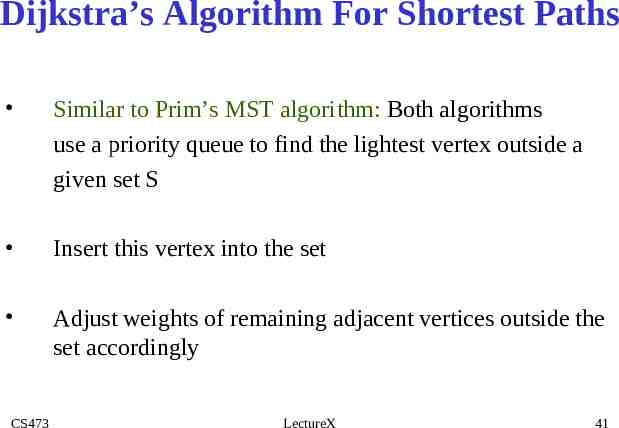
Dijkstra’s Algorithm For Shortest Paths Similar to Prim’s MST algorithm: Both algorithms use a priority queue to find the lightest vertex outside a given set S Insert this vertex into the set Adjust weights of remaining adjacent vertices outside the set accordingly CS473 LectureX 41
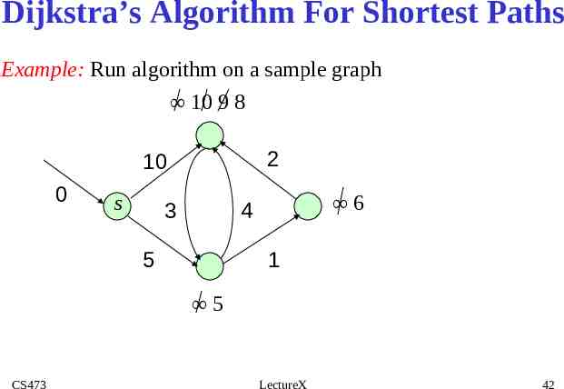
Dijkstra’s Algorithm For Shortest Paths Example: Run algorithm on a sample graph 10 9 8 2 10 0 s 3 6 4 5 1 5 CS473 LectureX 42
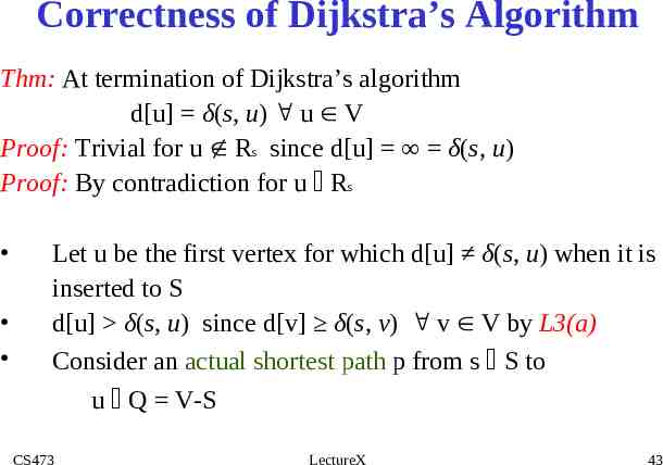
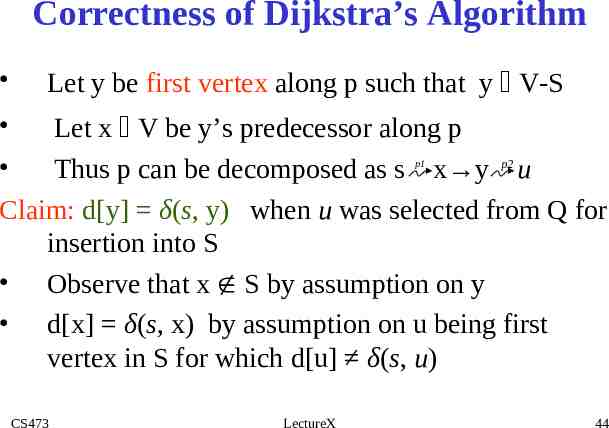
Correctness of Dijkstra’s Algorithm Thm: At termination of Dijkstra’s algorithm d[u] δ(s, u) u V Proof: Trivial for u Rs since d[u] δ(s, u) Proof: By contradiction for u Rs Let u be the first vertex for which d[u] δ(s, u) when it is inserted to S d[u] δ(s, u) since d[v] δ(s, v) v V by L3(a) Consider an actual shortest path p from s S to u Q V-S CS473 LectureX 43
Correctness of Dijkstra’s Algorithm Let y be first vertex along p such that y V-S Let x V be y’s predecessor along p Thus p can be decomposed as s x y p2 u Claim: d[y] δ(s, y) when u was selected from Q for insertion into S Observe that x S by assumption on y d[x] δ(s, x) by assumption on u being first vertex in S for which d[u] δ(s, u) p1 CS473 LectureX 44
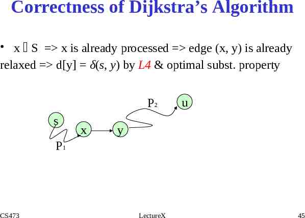
Correctness of Dijkstra’s Algorithm x S x is already processed edge (x, y) is already relaxed d[y] δ(s, y) by L4 & optimal subst. property P2 s x u y P1 CS473 LectureX 45
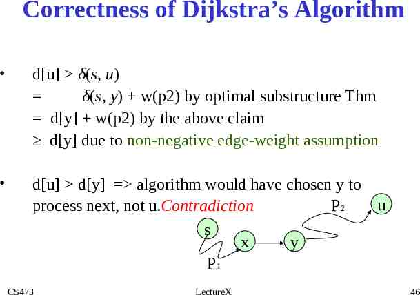
Correctness of Dijkstra’s Algorithm d[u] δ(s, u) δ(s, y) w(p2) by optimal substructure Thm d[y] w(p2) by the above claim d[y] due to non-negative edge-weight assumption d[u] d[y] algorithm would have chosen y to u P2 process next, not u.Contradiction s x y P1 CS473 LectureX 46
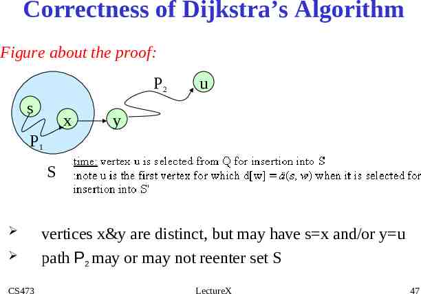
Correctness of Dijkstra’s Algorithm Figure about the proof: P2 s x u y P1 S CS473 vertices x&y are distinct, but may have s x and/or y u path P2 may or may not reenter set S LectureX 47
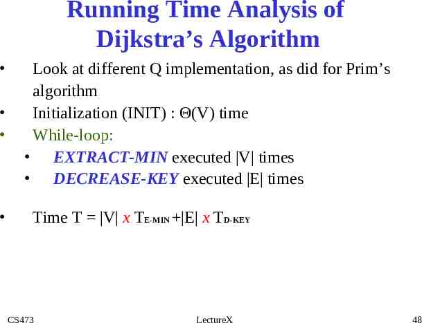
Running Time Analysis of Dijkstra’s Algorithm Look at different Q implementation, as did for Prim’s algorithm Initialization (INIT) : Θ(V) time While-loop: EXTRACT-MIN executed V times DECREASE-KEY executed E times Time T V x TE-MIN E x TD-KEY CS473 LectureX 48
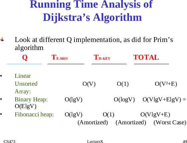
Running Time Analysis of Dijkstra’s Algorithm Look at different Q implementation, as did for Prim’s algorithm Q TE-MIN TD-KEY TOTAL Linear Unsorted Array: Binary Heap: O(ElgV) Fibonacci heap: CS473 O(V) O(lgV) O(1) O(V² E) O(logV) O(VlgV ElgV) O(lgV) O(1) O(VlgV E) (Amortized) (Amortized) (Worst Case) LectureX 49
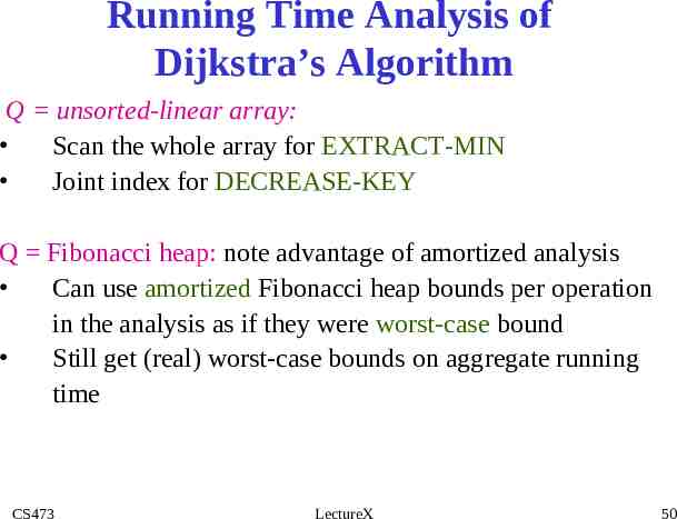
Running Time Analysis of Dijkstra’s Algorithm Q unsorted-linear array: Scan the whole array for EXTRACT-MIN Joint index for DECREASE-KEY Q Fibonacci heap: note advantage of amortized analysis Can use amortized Fibonacci heap bounds per operation in the analysis as if they were worst-case bound Still get (real) worst-case bounds on aggregate running time CS473 LectureX 50
Bellman-Ford Algorithm for Single Source Shortest Paths More general than Dijkstra’s algorithm: Edge-weights can be negative Detects the existence of negative-weight cycle(s) reachable from s. CS473 LectureX 51
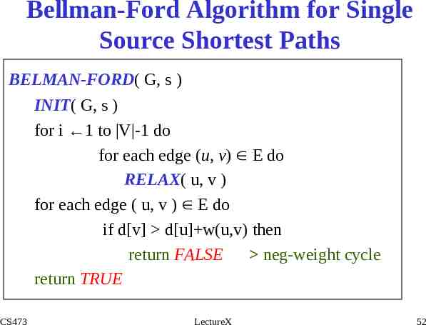
Bellman-Ford Algorithm for Single Source Shortest Paths BELMAN-FORD( G, s ) INIT( G, s ) for i 1 to V -1 do for each edge (u, v) E do RELAX( u, v ) for each edge ( u, v ) E do if d[v] d[u] w(u,v) then return FALSE neg-weight cycle return TRUE CS473 LectureX 52
Bellman-Ford Algorithm for Single Source Shortest Paths Observe: First nested for-loop performs V -1 relaxation passes; relax every edge at each pass Last for-loop checks the existence of a negative-weight cycle reachable from s CS473 LectureX 53
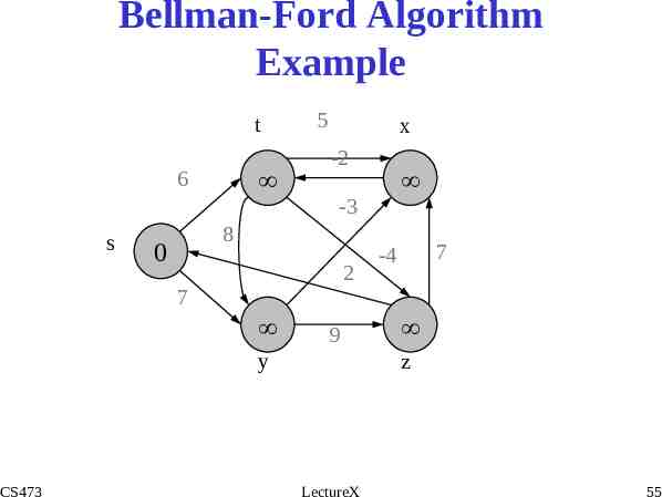
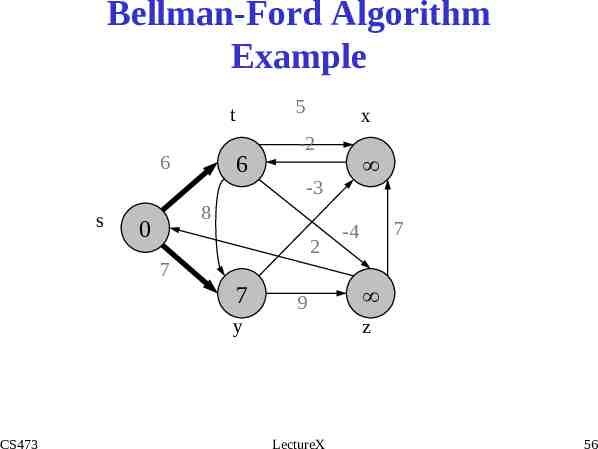
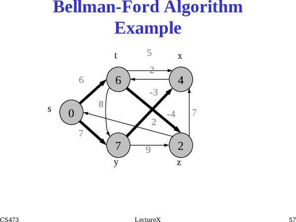
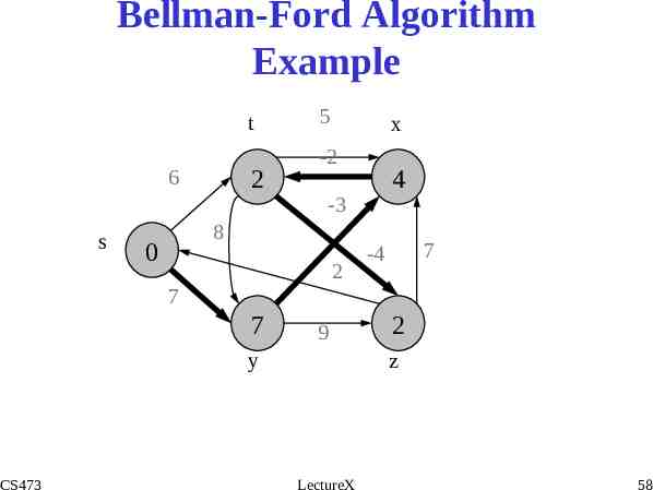
Bellman-Ford Algorithm for Single Source Shortest Paths CS473 Running time O(VxE) Constants are good; it’s simple, short code(very practical) Example: Run algorithm on a sample graph with no negative weight cycles. LectureX 54
Bellman-Ford Algorithm Example t x -2 6 s 5 -3 8 2 7 -4 7 9 y CS473 z LectureX 55
Bellman-Ford Algorithm Example 5 t -2 6 s x -3 8 2 7 -4 7 9 y CS473 z LectureX 56
Bellman-Ford Algorithm Example t x -2 6 s 5 -3 8 2 7 -4 7 9 y CS473 z LectureX 57
Bellman-Ford Algorithm Example t x -2 6 s 5 -3 8 2 7 -4 7 9 y CS473 z LectureX 58
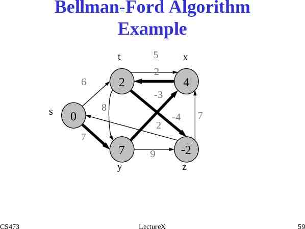
Bellman-Ford Algorithm Example t -3 8 x -2 6 s 5 2 7 -4 7 9 y CS473 z LectureX 59
Bellman-Ford Algorithm for Single Source Shortest Paths Converges in just 2 relaxation passes Values you get on each pass & how early converges depend on edge process order d value of a vertex may be updated more than once in a pass CS473 LectureX 60
Correctness of Bellman-Ford Algorithm L5: Assume that G contains no negative-weight cycles reachable from s Thm, at termination of BELLMAN-FORD, we have d[v] δ(s, v) v Rs Proof: Let v Rs , consider a shortest path p v0 s,v1,v2,.,vk v from s to v CS473 LectureX 61
Correctness of Bellman-Ford Algorithm No neg-weight cycle path p is simple k V -1 o i.e., longest simple path has V -1 edge prove by induction that for i 0,1,.,k o we have d[v1] δ(s,vi) after i-th pass and this equality maintained thereafter basis: d[v0 s] 0 δ(s, s) after INIT( G, s ) and doesn’t change by L3(b) hypothesis: assume that d[vi-1] δ(s,vi-1) after the (i-1)th pass CS473 LectureX 62
Correctness of Bellman-Ford Algorithm Edge (vi-1, vi) is relaxed in the ith pass o so by L4 , d[vi] δ(s,vi) after i-th pass, and doesn’t change thereafter Thm:Bellman-Ford algorithm (a) returns TRUE together with correct d values, if G contains no neg-weight cycle Rs (b) returns FALSE, otherwise CS473 LectureX 63
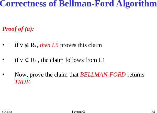
Correctness of Bellman-Ford Algorithm Proof of (a): if v Rs , then L5 proves this claim if v Rs , the claim follows from L1 Now, prove the claim that BELLMAN-FORD returns TRUE CS473 LectureX 64
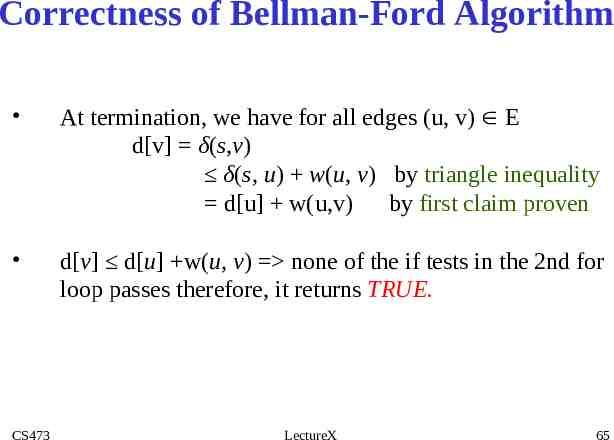
Correctness of Bellman-Ford Algorithm At termination, we have for all edges (u, v) E d[v] δ(s,v) δ(s, u) w(u, v) by triangle inequality d[u] w(u,v) by first claim proven d[v] d[u] w(u, v) none of the if tests in the 2nd for loop passes therefore, it returns TRUE. CS473 LectureX 65
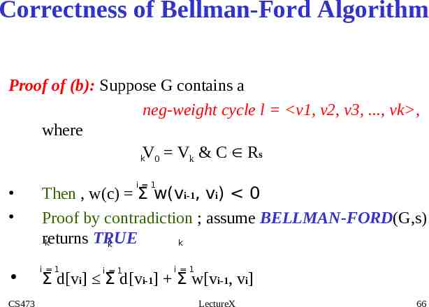
Correctness of Bellman-Ford Algorithm Proof of (b): Suppose G contains a neg-weight cycle l v1, v2, v3, ., vk , where kV0 Vk & C Rs i 1 Then , w(c) Σ w(vi-1, vi) 0 Proof by contradiction ; assume BELLMAN-FORD(G,s) returns TRUE k k k i 1 CS473 i 1 i 1 Σ d[vi] Σ d[vi-1] Σ w[vi-1, vi] LectureX 66
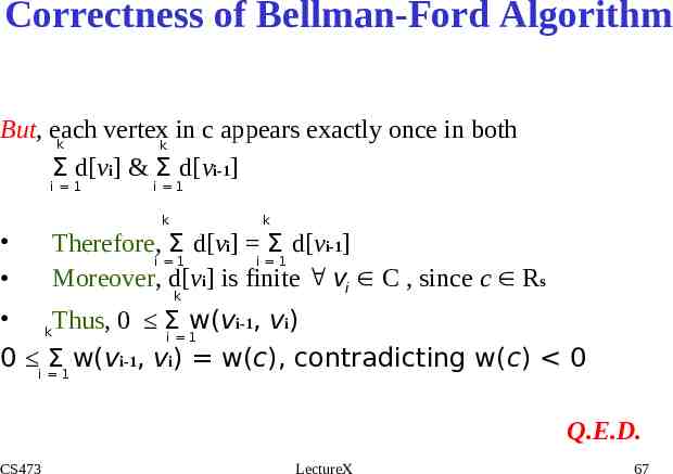
Correctness of Bellman-Ford Algorithm But, each vertexk in c appears exactly once in both k Σ d[vi] & Σ d[vi-1] i 1 i 1 k k Therefore, Σ d[vi] Σ d[vi-1] i 1 i 1 Moreover, d[vi] is finite vi C , since c Rs k Thus, 0 Σ w(vi-1, vi) i 1 0 i Σ1 w(vi-1, vi) w(c), contradicting w(c) 0 k Q.E.D. CS473 LectureX 67
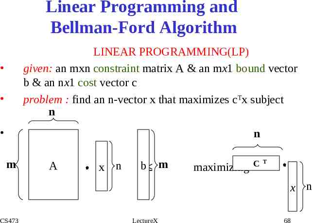
Linear Programming and Bellman-Ford Algorithm LINEAR PROGRAMMING(LP) given: an mxn constraint matrix A & an mx1 bound vector b & an nx1 cost vector c problem : find an n-vector x that maximizes cTx subject n n m A A x n b m maximizing C T x n CS473 LectureX 68
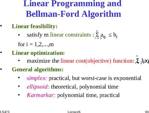
Linear Programming and Bellman-Ford Algorithm CS473 Linear feasibility: n satisfy m linear constraints : iΣ 1aij bi for i 1,2,.,m Linear optimization: n maximize the linear cost(objective) function: iΣ 1ljxj General algorithms: simplex: practical, but worst-case is exponential ellipsoid: theoretical, polynomial time Karmarkar: polynomial time, practical LectureX 69
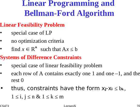
Linear Programming and Bellman-Ford Algorithm Linear Feasibility Problem special case of LP no optimization criteria n find x R such that Ax b Systems of Difference Constraints special case of linear feasibility problem each row of A contains exactly one 1 and one –1, and the rest 0 thus, constraints have the form xj-xi bk , 1 i, j n & 1 k m CS473 LectureX 70
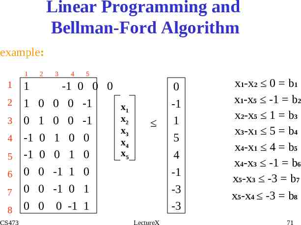
Linear Programming and Bellman-Ford Algorithm example: 1 1 2 3 4 5 6 7 8 CS473 1 1 0 -1 -1 0 0 0 2 0 1 0 0 0 0 0 3 4 5 -1 0 0 0 0 0 -1 x1 x2 0 0 -1 x3 1 0 0 x4 x5 0 1 0 -1 1 0 -1 0 1 0 -1 1 LectureX 0 -1 1 5 4 -1 -3 -3 x1-x2 0 b1 x1-x5 -1 b2 x2-x5 1 b3 x3-x1 5 b4 x4-x1 4 b5 x4-x3 -1 b6 x5-x3 -3 b7 x5-x4 -3 b8 71
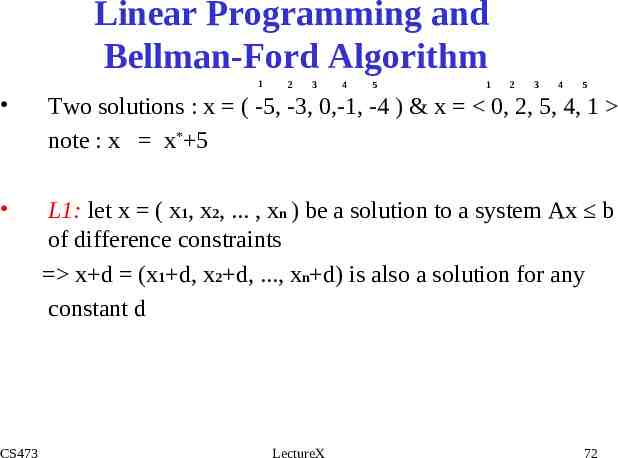
Linear Programming and Bellman-Ford Algorithm 1 2 3 4 5 1 2 3 4 5 Two solutions : x ( -5, -3, 0,-1, -4 ) & x 0, 2, 5, 4, 1 note : x x* 5 L1: let x ( x1, x2, . , xn ) be a solution to a system Ax b of difference constraints x d (x1 d, x2 d, ., xn d) is also a solution for any constant d CS473 LectureX 72
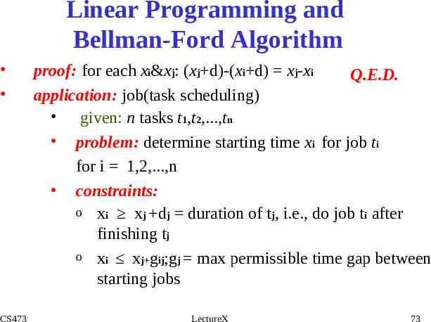
Linear Programming and Bellman-Ford Algorithm CS473 proof: for each xi&xj: (xj d)-(xi d) xj-xi Q.E.D. application: job(task scheduling) given: n tasks t1,t2,.,tn problem: determine starting time xi for job ti for i 1,2,.,n constraints: o xi xj dj duration of tj, i.e., do job ti after finishing tj o xi xj gij;gj max permissible time gap between starting jobs LectureX 73
Linear Programming and Bellman-Ford Algorithm graph theoritical representation of difference constraints a system Ax b of difference constraints with an mxn constraint matrix A incidence matrix of an edge-weighted directed graph with n vertices and m edges CS473 one vertex per variable: V {v1,v2,.,vn} such that Vi Xi for i 1,2,.,n LectureX 74
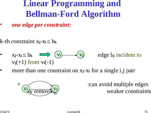
Linear Programming and Bellman-Ford Algorithm one edge per constraint: k-th constraint xj-xi bk vi vj xj-xi bk edge lij incident to vj( 1) from vi(-1) more than one constraint on xj-xi for a single i,j pair o CS473 :can avoid multiple edges weaker constraints vby i vj removing LectureX 75
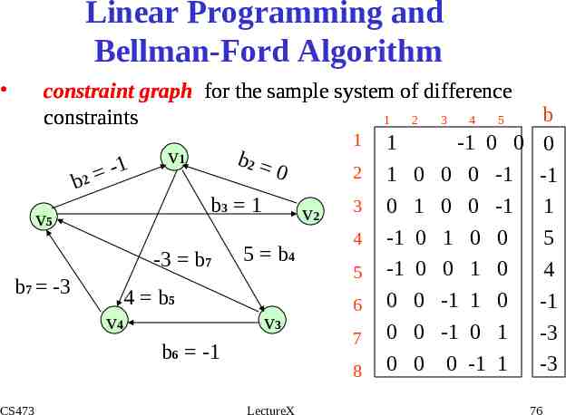
Linear Programming and Bellman-Ford Algorithm constraint graph for the sample system of difference constraints 1 2 3 4 5 1 1 -1 0 0 v 1 b2 1 0 2 1 0 0 0 -1 b2 3 0 1 0 0 -1 b3 1 v 2 v5 4 -1 0 1 0 0 -3 b7 5 b4 5 -1 0 0 1 0 b7 -3 4 b5 6 0 0 -1 1 0 v4 v3 7 0 0 -1 0 1 b6 -1 8 0 0 0 -1 1 CS473 LectureX b 00 -1 1 5 4 -1 -3 -3 76
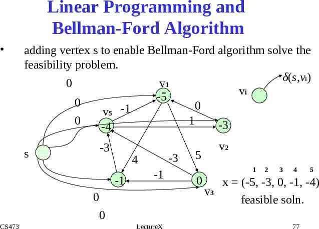
Linear Programming and Bellman-Ford Algorithm adding vertex s to enable Bellman-Ford algorithm solve the feasibility problem. δ(s,vi) 0 v1 vi -5 0 0 v5 -1 0 1 -3 -4 s -3 -3 4 -1 -1 0 0 CS473 LectureX 5 v2 1 0 2 3 4 5 x (-5, -3, 0, -1, -4) v3 feasible soln. 77
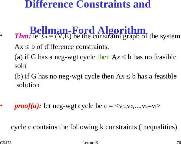
Difference Constraints and Bellman-Ford Algorithm Thm: let G (V,E) be the constraint graph of the system Ax b of difference constraints. (a) if G has a neg-wgt cycle then Ax b has no feasible soln (b) if G has no neg-wgt cycle then Ax b has a feasible solution proof(a): let neg-wgt cycle be c v1,v2,.,vk vl cycle c contains the following k constraints (inequalities) CS473 LectureX 78
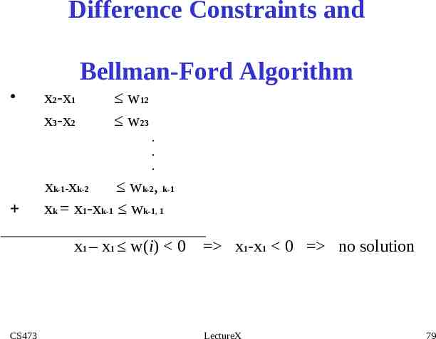
Difference Constraints and Bellman-Ford Algorithm x2-x1 x3-x2 w12 w23 . . . xk-1-xk-2 wk-2, k-1 xk x1-xk-1 wk-1, 1 x1 – x1 w(i) 0 CS473 x1-x1 0 no solution LectureX 79
Difference Constraints and Bellman-Ford Algorithm Consider any feasible soln. x for Ax b o x must satisfy each of these k inequalities o x must also satisfy the inequality that results when we sum them together CS473 LectureX 80
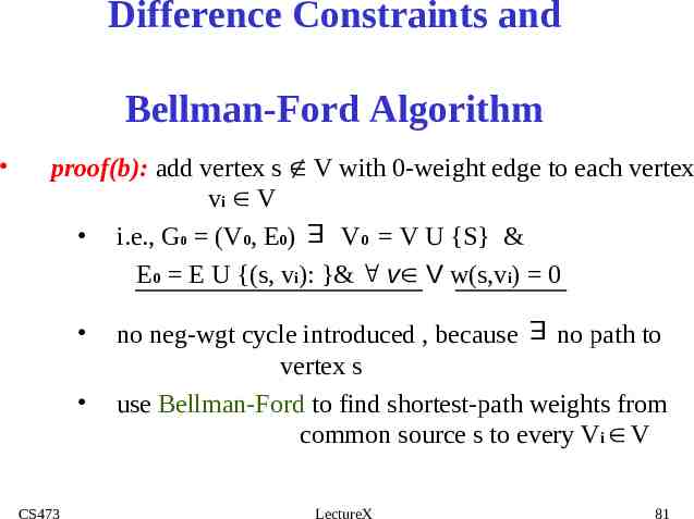
Difference Constraints and Bellman-Ford Algorithm proof(b): add vertex s V with 0-weight edge to each vertex vi V i.e., G0 (V0, E0) V0 V U {S} & E0 E U {(s, vi): }& v V w(s,vi) 0 E CS473 E no neg-wgt cycle introduced , because no path to vertex s use Bellman-Ford to find shortest-path weights from common source s to every Vi V LectureX 81
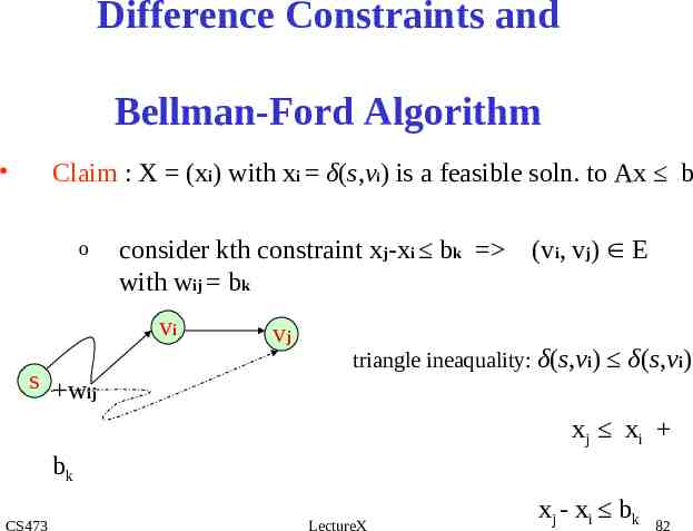
Difference Constraints and Bellman-Ford Algorithm Claim : X (xi) with xi δ(s,vi) is a feasible soln. to Ax b o consider kth constraint xj-xi bk (vi, vj) E with wij bk vi s wij vj triangle ineaquality: δ(s,vi) δ(s,vi) xj xi bk CS473 LectureX xj - xi bk 82
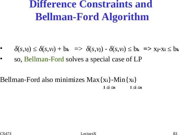
Difference Constraints and Bellman-Ford Algorithm δ(s,vj) δ(s,vi) bk δ(s,vj) - δ(s,vi) bk xj-xi bk so, Bellman-Ford solves a special case of LP Bellman-Ford also minimizes Max{xi}-Min{xi} 1 i n CS473 LectureX 1 i n 83