Basics of Supply Chain Management Dr Avinash Desai B.Sc,MBA,PhD,


31 Slides299.21 KB
Basics of Supply Chain Management Dr Avinash Desai B.Sc,MBA,PhD, Fellow Member – IIMM, Mumbai
Definitions
What Is the Supply Chain? Also referred to as the logistics network Suppliers, manufacturers, warehouses, distribution centers and retail outlets – “facilities” and the Raw materials Work-in-process (WIP) inventory Finished products that flow between the facilities
History of Supply Chain Management Before 1960 Focus on Mass Production 1960 - 1970 - Inventory Management Focus, MRP & BOM Operations Planning Cost Control 1980’s - MRPII, JIT - Materials Management, Logistics, Cost Reduction 1990’s - SCM - ERP - “Integrated” Purchasing, Financials, Manufacturing, Order Entry TQM 2000’s - Optimized “Value Network” with Real-Time Decision Support; Synchronized & Collaborative Extended Network
The Supply Chain System Suppliers Manufacturers Warehouses &Customer Distribution Centers Material Costs Transportation Transportation Transportation Costs Costs Manufacturing Costs Inventory Costs Costs
The Supply Chain – Another View Plan Plan Source Source Suppliers Material Costs Make Make Manufacturers Buy Buy Deliver Deliver Warehouses & Distribution Centers Customers Transportation Transportation Costs Costs Transportation Manufacturing Costs Inventory Costs Costs
What Is Supply Chain Management (SCM)? Plan Source Make Deliver A set of approaches used to efficiently integrate – – – – Suppliers Manufacturers Warehouses Distribution centers So that the product is produced and distributed – – – In the right quantities To the right locations And at the right time System-wide costs are minimized and Service level requirements are satisfied Buy
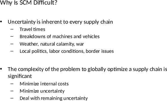
Why Is SCM Difficult? Uncertainty is inherent to every supply chain – – – – Travel times Breakdowns of machines and vehicles Weather, natural calamity, war Local politics, labor conditions, border issues The complexity of the problem to globally optimize a supply chain is significant – – – Minimize internal costs Minimize uncertainty Deal with remaining uncertainty
The Importance of Supply Chain Management Dealing with uncertain environments – matching supply and demand – – – – Boeing announced a 2.6 billion write-off in 1997 due to “raw materials shortages, internal and supplier parts shortages and productivity inefficiencies” U.S Surgical Corporation announced a 22 million loss in 1993 due to “larger than anticipated inventories on the shelves of hospitals” IBM sold out its supply of its new Aptiva PC in 1994 costing it millions in potential revenue Hewlett-Packard and Dell found it difficult to obtain important components for its PC’s from Taiwanese suppliers in 1999 due to a massive earthquake U.S. firms spent 898 billion (10% of GDP) on supply-chain related activities in 1998
The Importance of Supply Chain Management Shorter product life cycles of high-technology products – – Less opportunity to accumulate historical data on customer demand Wide choice of competing products makes it difficult to predict demand The growth of technologies such as the Internet enable greater collaboration between supply chain trading partners – – If you don’t do it, your competitor will Major buyers such as Wal-Mart demand a level of “supply chain maturity” of its suppliers Availability of SCM technologies on the market – Firms have access to multiple products (e.g., SAP, Baan, Oracle, JD Edwards) with which to integrate internal processes
Supply Chain Management and Uncertainty Inventory and back-order levels fluctuate considerably across the supply chain even when customer demand doesn’t vary The variability deteriorate as we travel “up” the supply chain Forecasting doesn’t help! Wholesale Distributor s Time Consum ers Sales Sales Time Retaile rs Sales Manufactu rer Sales Multi-tier Suppliers Time Bullwhip Effect Time
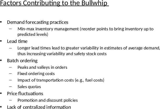
Factors Contributing to the Bullwhip Demand forecasting practices – Min-max inventory management (reorder points to bring inventory up to predicted levels) Lead time – Longer lead times lead to greater variability in estimates of average demand, thus increasing variability and safety stock costs Batch ordering – – – – Peaks and valleys in orders Fixed ordering costs Impact of transportation costs (e.g., fuel costs) Sales quotas Price fluctuations – Promotion and discount policies Lack of centralized information
Fourth Party Logistics: The Evolution of Supply Chain Outsourcing
Outline 1. Outsourcing: Third Party Logistics W hy outsourcing Outsourcing logisticsfunctions, but which? 2. Fourth Party Logistics(4PL) Definition Example 3 types of4PL
Outline 3. Technology inthe next generation of Supply Chain Outsourcing 4. Supply Chain Value Proposition Revenue Enhancement Operating Cost Reduction WorkingCapital Reduction Fixed Capital Reduction 5. Potentials and Constrains
Inventory Management Models
Inventory Management Models Deterministic ( Models assuming certainty ) Fixed Quantity ( perpetual Inventory system ) Fixed Period ( Periodic Inventory System ) Probabilistic ( Stochastic ) ( Models Assuming Risk ) Fixed Quantity System Fixed period System
DETERMINISTIC MODELS The Following assumptions are made in Deterministic models: Demand is known exactly for a given period. Demand is uniform and constant over a period of time. No, imitations are imposed by strong capacity and clerical capacity. The cost of an order and storing a unit of material are independent of the order quantity. Order are received instantaneously. Order and delivery quantities are Equal. Buffer Stock of finished product is independent of order quantity. Price of Raw – material are stable. Ordering cost are the same regardless of order size. Similarly set up costs are constant and the rate at which products are produced in known.
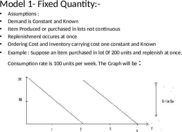
Model 1- Fixed Quantity: Assumptions : Demand is Constant and Known Item Produced or purchased in lots not continuous Replenishment occures at once Ordering Cost and Inventory carrying cost one constant and Known Example : Suppose an item purchased in lot 0f 200 units and replenish at once. Consumption rate is 100 units per week. The Graph will be :
Cost Order Size Relationship
To Find Out :Q Average Inventory : -------2 Annual demand Number of orders per year ----------------------Order quantity RELEVANT COST : Annual cost of Placing Orders Annual cost of Carrying Inventory LET : A Annual consumption in units S Ordering cost per year , C Unit cost, i Annual carrying cost, as decimal of percentage Q Order quantity in units ( A.) Annual Ordering Cost : No. of orders X cost per order Annual demand ---------------------- X Cost per order Order quantity A ----- X S Q
( B.) Annual Carrying Inventory : Average Inventory X Cost of carrying one unit for one year Average Inventory X unit cost X carrying cost Q ------ X C X i 2 Total Annual Cost Annual ordering cost annual Carrying cost A Q ---- X S ------ X C X i Q 2 E OQ ordering cost Carrying cost AS QCi ------ ------Q 2 2 AS Q2 C i 2AS 2 Q --------Ci Q 2 A S / C i
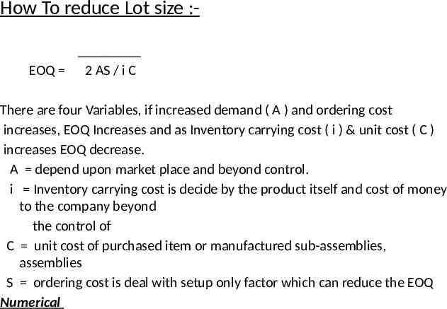
How To reduce Lot size : EOQ 2 AS / i C There are four Variables, if increased demand ( A ) and ordering cost increases, EOQ Increases and as Inventory carrying cost ( i ) & unit cost ( C ) increases EOQ decrease. A depend upon market place and beyond control. i Inventory carrying cost is decide by the product itself and cost of money to the company beyond the control of C unit cost of purchased item or manufactured sub-assemblies, assemblies S ordering cost is deal with setup only factor which can reduce the EOQ Numerical
MODEL 2 : EOQ for Lots :If a product is produced at one stage, stored as an inventory, and then transmitted to the customers. In other words, when the rate of flow of Inventory is greater than the demand rate, this model is most appropriate for determining the size of Lots. Assumptions are : 1. Annual demand, carrying cost, and ordering /pro amount cost for a material / product can be estimated. 2. No safety stock is utilized, goods one supplied at a uniform rate( P ) and used at a uniform rate ( d ) 3. Goods one entirely used up when the next order begins to arrive. 4. Stock out, customer responsibilities, and other cost have no effect. 5. Quantity discount do not exist. 6. Supply rate ( P ) is greater than usage rate ( d ) Let :D Annual demand Q Order quantity in units. C Annual carrying cost of one unit ( Rs./Unit/year ) S Average cost of per order per year d Rate of which units used / consume from inventory ( units per time period) P rate of which units are supplied to Inventory. Maximum Inventory Level Inventory build up rate X period of delivery Minimum Inventory level 0 ( Zero )
Hence :- Q Maximum Inventory Level ( P – d ) X -----P Maximum Inventory Level Minimum Inventory Level Average Inventory Level ---------------------------------------------------------------------------2 ( P – d ) ( Q/P) 0 -----------------------2 ( P – d ) ( Q/P ) -------------------2 PQ – dQ Average Inventory level ---------2P Q P–d ----- ------- 2 P
Annual carrying Cost Average Inventory X carrying cost Q P–d ---- ( --------- ) 2 P XC Annual Ordering cost orders per year X ordering cost D ------- X S Q Total Annual stock cost Annual carrying cost annual ordering cost For EOQ Q Q P–d ---- ( --------- ) X C 2 P 2 D S P ( -------- ) ( --------- ) C P–d D ------ X S Q
Model : 2 ( EOQ For Lots )
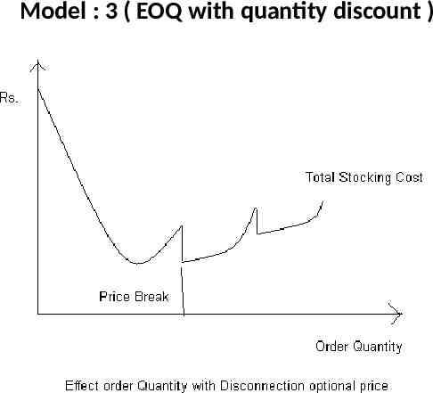
Model : 3 ( EOQ with quantity discount )
When material is purchased, supplier offer discount on order a certain size. The buyer must decide whether to accept the discount. Before accepting must consider the relevant cost :( a ) Purchase cost (b ) Ordering Cost ( c ) Carrying Cost Example : - An Item has an annual demand of 25,000 units, a unit cost is Rs. 10, an order preparation cost is Rs. 10, and a carrying cost of 20%. It is ordered on the basis of EOQ. But the supplier has offered, a discount of 2% on order of Rs. 10,000 or more. Should the offer be accepted ? Solution :- EOQ 2 ADS / i 2 X ( 25,000 X 10 ) X 10 / 0.2 As A D demand in value hence 25,000 X 10 Rs. 5,000/As supplier offer discount on the value of Rs. 10,000 or more. Hence on discount EOQ 10,000 X 2% Rs. 9800/-
To Find out the best offer, need to calculate purchase cost, ordering cost and carrying cost. Hence : Sr. No. Particulars Discount No discount 1. Unit Price Rs. 9.80/- Rs. 10.00/- 2. Lot Size ( As Calculated from EOQ ) Rs. 9800/- Rs. 5,000/- 3. Average Lot size ( Q/2 ) Rs. 9800/2 Rs. 4900/- Rs. 5000/2 Rs. 2500/- 4. No. of Orders per Year Annual demand ---------------------Order qty 25000 25000 ------------- 25.51 ------------- 50/(5000/10) (9800/10)
( As order quantity calculated in value of Rs. Hence, EOQ is Divide by unit price to get value in units ) Now Calculated :Sr. No. 1. 2. 3. Particulars Purchase cost ( demand X value per unit ) Ordering cost ( A/Q X S ) Carrying Cost ( Q/2 X C X i ) No Need to multiply unit price, because value already calculated in Rs. Discount No discount 2,45,000/- 2,50,000/- 255/- 250/- 4900 X 20% 980/- 2500 X 205 500/- Total Value :- ( A ) Discounted 2,45,500 255 980 2,46,735/( B ) No Discount 2,50,000 250 500 2,50,750/From the above Solution :1. There is saving in Purchase cost 2. Inventory carrying cost increase because large quantity ordered 3. Ordering Cost reduced, because few order placed with large quantity.