AG C Power Spectral Estimation DS P The purpose of these methods
30 Slides294.50 KB
AG C Power Spectral Estimation DS P The purpose of these methods is to obtain an approximate estimation of the j power spectral density yy (e ) of a given real random process { yn } RAVI KISHORE 1
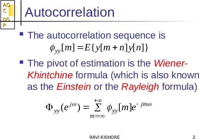
AG C Autocorrelation DS P The autocorrelation sequence is yy [m] E{ y[m n] y[n]} The pivot of estimation is the WienerKhintchine formula (which is also known as the Einstein or the Rayleigh formula) j yy (e ) yy [m]e jm m RAVI KISHORE 2
AG C Classification DS P The crux of PSD estimation is the determination of the autocorrelation sequence from a given process. Methods that rely on the direct use of the given finite duration signal to compute the autocorrelation to the maximum allowable length (beyond which it is assumed zero), are called Non-parametric methods Methods that rely on a model for the signal generation are called Modern or Parametric methods. Personally I prefer the names “Direct” and “Indirect Methods” RAVI KISHORE 3
AG C Classification & Choice DS P The choice between the two options is made on a balance between “simple and fast computations but inaccurate PSD estimates” Vs “computationally involved procedures but enhanced PSD estimates” RAVI KISHORE 4
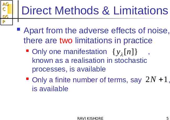
AG C Direct Methods & Limitations DS P Apart from the adverse effects of noise, there are two limitations in practice Only one manifestation { y [n]} , known as a realisation in stochastic processes, is available Only a finite number of terms, say 2 N 1 , is available RAVI KISHORE 5
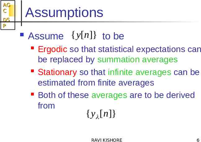
AG C Assumptions DS P Assume { y[n]} to be Ergodic so that statistical expectations can be replaced by summation averages Stationary so that infinite averages can be estimated from finite averages Both of these averages are to be derived from { y [n]} RAVI KISHORE 6
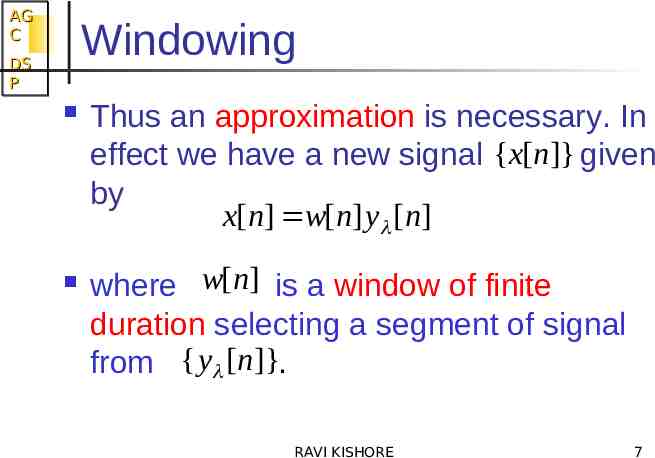
AG C Windowing DS P Thus an approximation is necessary. In effect we have a new signal {x[n]} given by x[n] w[n] y [n] where w[n] is a window of finite duration selecting a segment of signal from { y [n]}. RAVI KISHORE 7
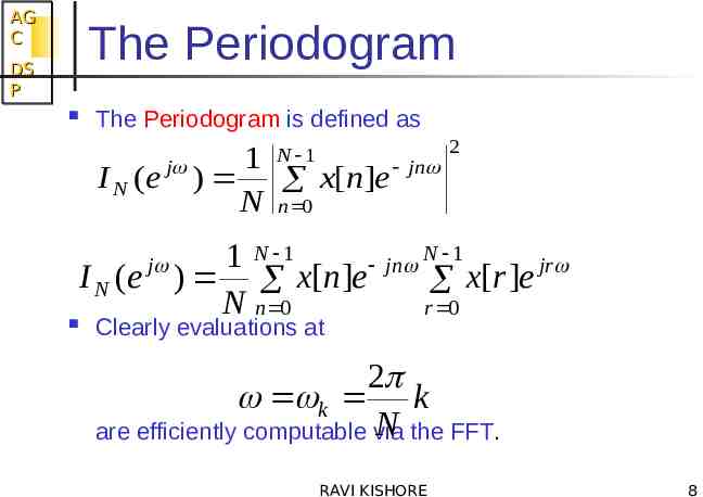
AG C The Periodogram DS P The Periodogram is defined as 1 N 1 j I N (e ) x[n]e N n 0 jn 2 N 1 1 N 1 jn jr I N (e ) x[n]e x[r ]e N n 0 r 0 j Clearly evaluations at 2 k k N the FFT. are efficiently computable via RAVI KISHORE 8
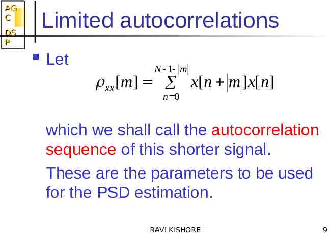
AG C Limited autocorrelations DS P Let N 1 m xx [m] x[n m ]x[n] n 0 which we shall call the autocorrelation sequence of this shorter signal. These are the parameters to be used for the PSD estimation. RAVI KISHORE 9
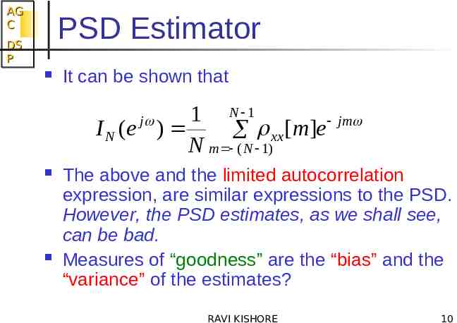
AG C PSD Estimator DS P It can be shown that 1 N 1 jm I N (e ) [ m ] e xx N m ( N 1) j The above and the limited autocorrelation expression, are similar expressions to the PSD. However, the PSD estimates, as we shall see, can be bad. Measures of “goodness” are the “bias” and the “variance” of the estimates? RAVI KISHORE 10
AG C The Bias DS P The Bias pertains to the question: Does the estimate tend to the correct value as the number of terms taken tends to infinity? If yes, then it is unbiased, else it is biased. RAVI KISHORE 11
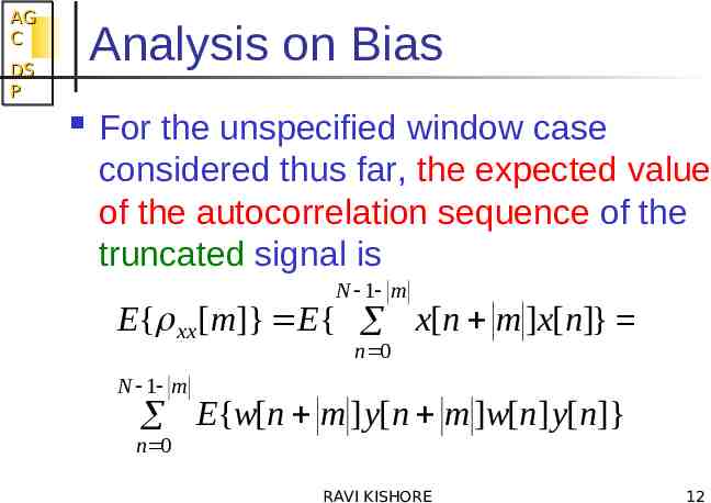
AG C Analysis on Bias DS P For the unspecified window case considered thus far, the expected value of the autocorrelation sequence of the truncated signal is N 1 m E{ xx [m]} E{ x[n m ]x[n]} n 0 N 1 m E{w[n m ] y[n m ]w[n] y[n]} n 0 RAVI KISHORE 12
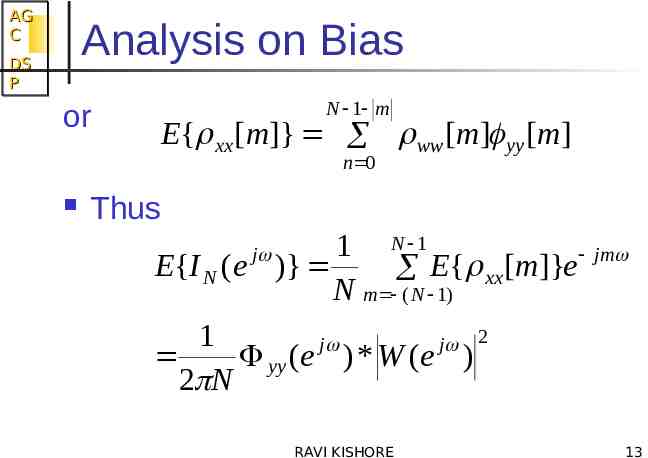
AG C Analysis on Bias DS P or N 1 m E{ xx [m]} ww [m] yy [m] n 0 Thus 1 N 1 jm E{I N (e )} E { [ m ]} e xx N m ( N 1) 1 j j 2 yy (e ) * W (e ) 2 N j RAVI KISHORE 13
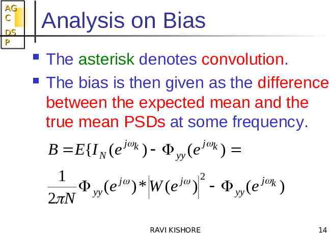
AG C Analysis on Bias DS P The asterisk denotes convolution. The bias is then given as the difference between the expected mean and the true mean PSDs at some frequency. B E{I N (e j k ) yy (e j k ) 1 j j 2 yy (e ) * W (e ) yy (e j k ) 2 N RAVI KISHORE 14
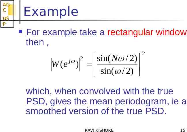
AG C Example DS P For example take a rectangular window then , sin( N / 2) W (e ) sin( / 2 ) j 2 2 which, when convolved with the true PSD, gives the mean periodogram, ie a smoothed version of the true PSD. RAVI KISHORE 15
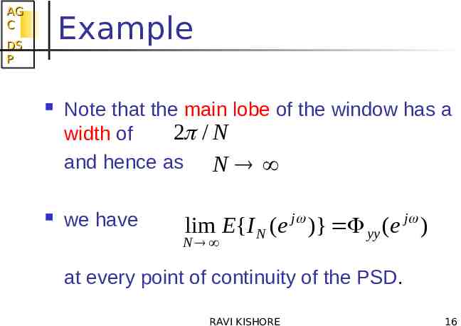
AG C Example DS P Note that the main lobe of the window has a 2 / N width of and hence as N we have j j lim E{I N (e )} yy (e ) N at every point of continuity of the PSD. RAVI KISHORE 16
AG C Asymptotically unbiased DS P j Thus I N (e ) is an asymptotically unbiased estimator of the true PSD. The result can be generalised as follows. RAVI KISHORE 17
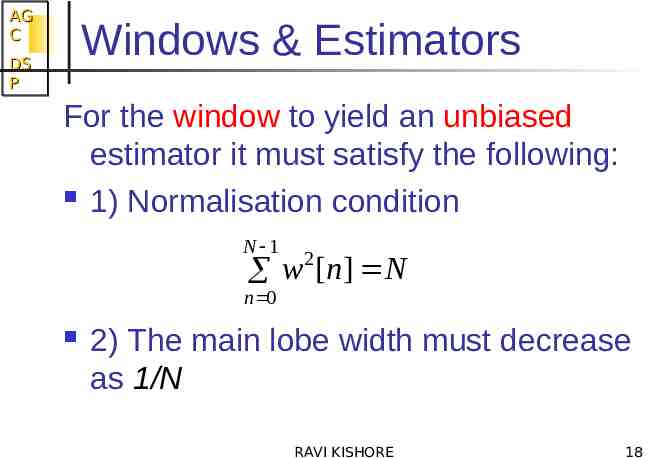
AG C Windows & Estimators DS P For the window to yield an unbiased estimator it must satisfy the following: 1) Normalisation condition N 1 2 w [ n] N n 0 2) The main lobe width must decrease as 1/N RAVI KISHORE 18
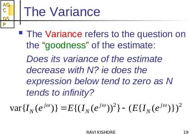
AG C The Variance DS P The Variance refers to the question on the “goodness” of the estimate: Does its variance of the estimate decrease with N? ie does the expression below tend to zero as N tends to infinity? j j 2 j var{I N (e )} E{( I N (e )) } ( E{I N (e )}) RAVI KISHORE 2 19
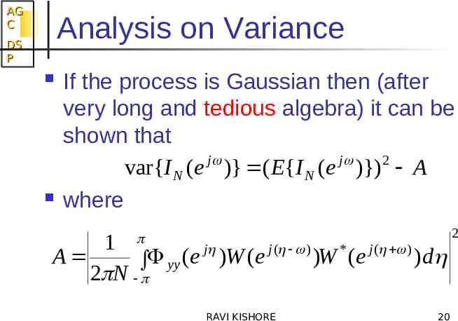
AG C Analysis on Variance DS P If the process is Gaussian then (after very long and tedious algebra) it can be shown that j j 2 var{I N (e )} ( E{I N (e )}) A where 1 j j ( ) * j ( ) A ( e ) W ( e ) W ( e )d yy 2 N RAVI KISHORE 20 2
AG C Analysis DS P Hence it is evident that as the length of data tends to infinity the first term remains unaffected, and thus the periodogram is an inconsistent estimator of the PSD. RAVI KISHORE 21
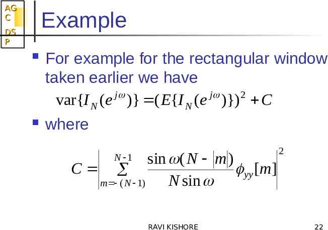
AG C Example DS P For example for the rectangular window taken earlier we have j j 2 var{I N (e )} ( E{I N (e )}) C where sin ( N m ) C yy [m] N sin m ( N 1) N 1 RAVI KISHORE 2 22
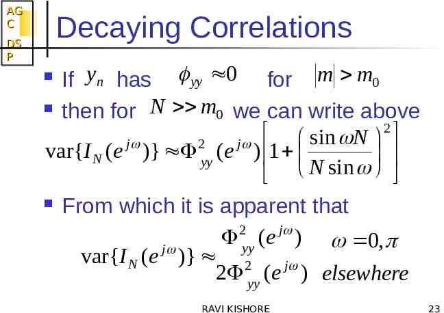
AG C DS P Decaying Correlations If yn has yy 0 for m m0 then for N m0 we can write above 2 sin N j 2 j var{I N (e )} yy (e ) 1 N sin From which it is apparent that 2 j yy (e ) 0, j var{I N (e )} 2 j 2 yy (e ) elsewhere RAVI KISHORE 23
AG C DS P Variance is large Thus even for very large windows the variance of the estimate is as large as the quantity to be estimated! RAVI KISHORE 24
AG C Smoothed Periodograms DS P Periodograms are therefore inadequate for precise estimation of a PSD. To reduce variance while keeping estimation simplicity and efficiency, several modifications can be implemented a) Averaging over a set of periodograms of (nearly) independent segments b) Windowing applied to segments c) Overlapping the windowed segments for additional averaging RAVI KISHORE 25
AG C DS P Welch-Bartlett Procedure Typical is the Welch-Bartlett procedure as follows. Let yn be an ergodic process from which we are given M data points for the signal y[n] . 1) Divide the given signal into K M / N blocks each of length N . 2) Estimate the PSD of each block 3) Take the average of these estimates RAVI KISHORE 26
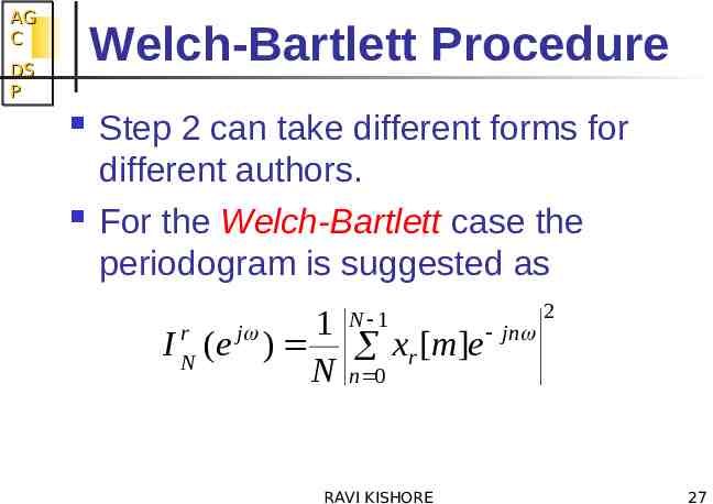
AG C Welch-Bartlett Procedure DS P Step 2 can take different forms for different authors. For the Welch-Bartlett case the periodogram is suggested as r IN 1 jn (e ) xr [m]e N n 0 j N 1 RAVI KISHORE 2 27
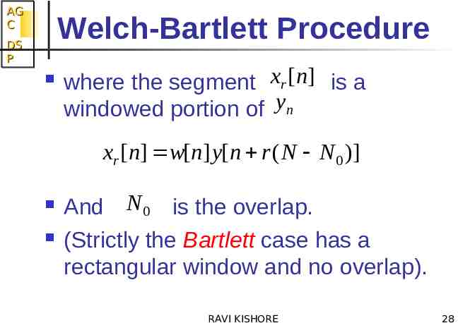
AG C Welch-Bartlett Procedure DS P where the segment xr [n] is a windowed portion of yn xr [n] w[n] y[n r ( N N 0 )] And N 0 is the overlap. (Strictly the Bartlett case has a rectangular window and no overlap). RAVI KISHORE 28
AG C Comments DS P FFT-based Spectral estimation is limited by a) the correlation assumed to be zero beyond the measurement length and b) the resolution attributes of the DFT. Thus if two frequencies are separated by then a data record of length N 2 / is required. (Uncertainty Principle) RAVI KISHORE 29
AG C Narrowband Signals DS P The spectrum to be estimated is some cases may contain narrow peaks (high Q resonances) as in speech formants or passive sonar. The limit on resolution imposed by window length is problematic in that it causes bias. The derived variance formulae are not accurate RAVI KISHORE 30