Radial Basis Function Networks 1. Introduction 2. Finding RBF

Radial Basis Function Networks 1. Introduction 2. Finding RBF Parameters 3. Decision Surface of RBF Networks 4. Comparison between RBF and BP 01/16/23 RBF Networks M.W. Mak

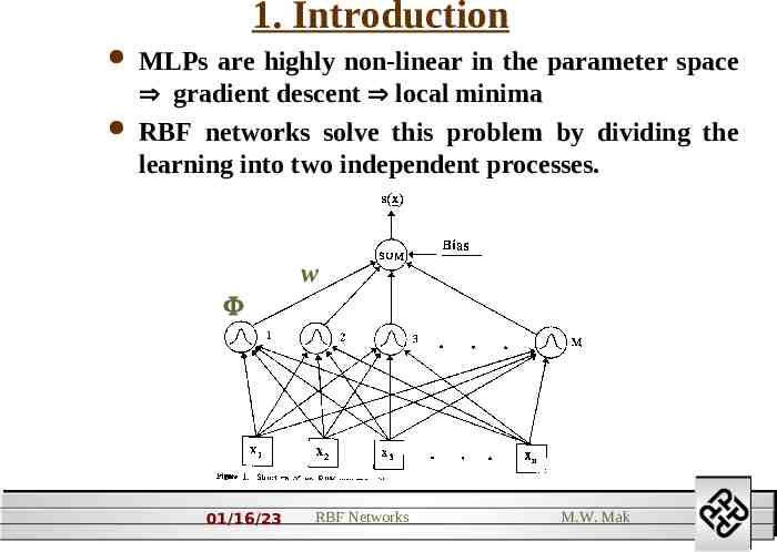
1. Introduction MLPs are highly non-linear in the parameter space gradient descent local minima RBF networks solve this problem by dividing the learning into two independent processes. w 01/16/23 RBF Networks M.W. Mak

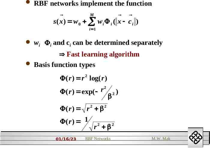
RBF networks implement the function M s( x ) w 0 w i i ( x c i ) i 1 wi i and ci can be determined separately Fast learning algorithm Basis function types ( r ) r 2 log( r ) 2 r ( r ) exp( 2 ) (r ) r 2 2 (r ) 1 01/16/23 r2 2 RBF Networks M.W. Mak

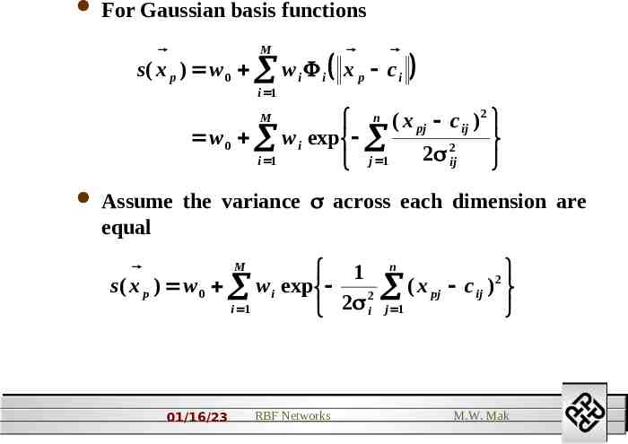
For Gaussian basis functions M s( x p ) w 0 w i i x p c i i 1 n ( x pj c ij ) 2 w 0 w i exp 2 2 ij i 1 j 1 M Assume the variance across each dimension are equal M 1 s( x p ) w 0 w i exp 2 2 i 1 i 01/16/23 RBF Networks n ( x pj c ij ) j 1 2 M.W. Mak

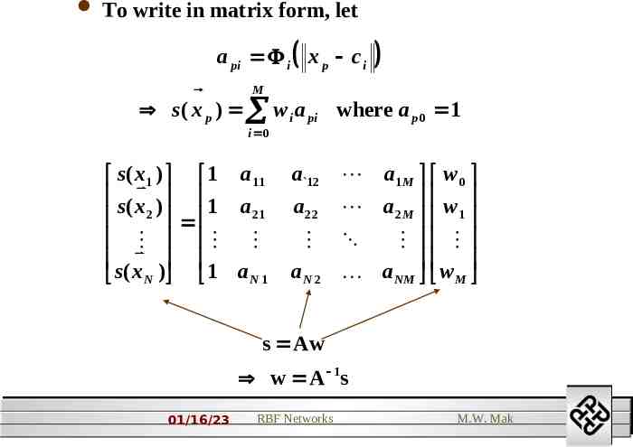
To write in matrix form, let a pi i x p c i M s( x p ) w i a pi where a p 0 1 i 0 s( x1 ) 1 a11 s( x ) 1 a 2 21 s( x ) 1 a N N1 a 12 a22 aN 2 a1 M w 0 a2 M w 1 a NM w M s Aw w A 1s 01/16/23 RBF Networks M.W. Mak

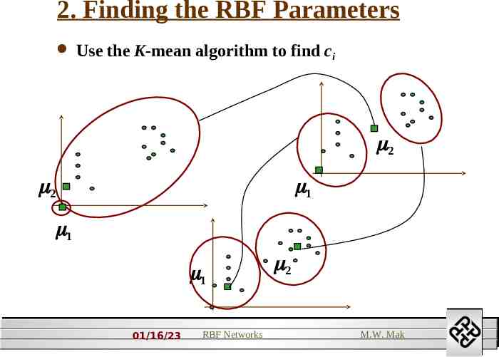
2. Finding the RBF Parameters Use the K-mean algorithm to find ci 2 2 1 1 1 01/16/23 RBF Networks 2 M.W. Mak

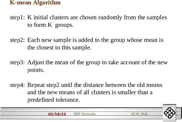
K-mean Algorithm step1: K initial clusters are chosen randomly from the samples to form K groups. step2: Each new sample is added to the group whose mean is the closest to this sample. step3: Adjust the mean of the group to take account of the new points. step4: Repeat step2 until the distance between the old means and the new means of all clusters is smaller than a predefined tolerance. 01/16/23 RBF Networks M.W. Mak

Outcome: There are K clusters with means representing the centroid of each clusters. Advantages: (1) A fast and simple algorithm. (2) Reduce the effects of noisy samples. 01/16/23 RBF Networks M.W. Mak

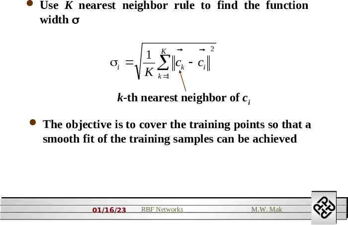
Use K nearest neighbor rule to find the function width 1 i K K ck ci 2 k 1 k-th nearest neighbor of ci The objective is to cover the training points so that a smooth fit of the training samples can be achieved 01/16/23 RBF Networks M.W. Mak

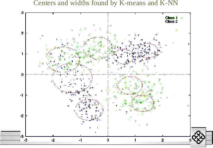
Centers and widths found by K-means and K-NN 01/16/23 RBF Networks M.W. Mak 1

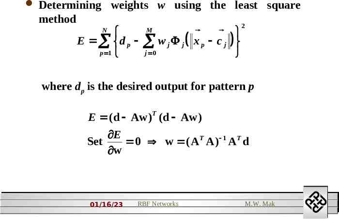
Determining weights w using the least square method 2 N M E d p w j j x p c j p 1 j 0 where dp is the desired output for pattern p E ( d Aw )T ( d Aw ) Set E 0 w ( A T A ) 1 A T d w 01/16/23 RBF Networks M.W. Mak 1

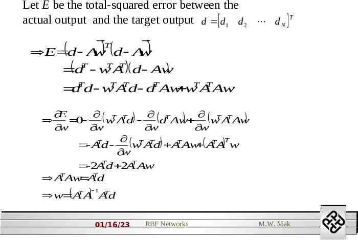
Let E be the total-squared error between the actual output and the target output d d1 d 2 d N T T E d Aw d Aw dT wTAT d Aw dTd wTATd dTAw wTATAw E T T T 0 w A d d Aw wTATAw w w w w T T T T T T A d w A d A Aw A A w w 2ATd 2ATAw ATAw ATd 1 w ATA ATd 01/16/23 RBF Networks M.W. Mak 1

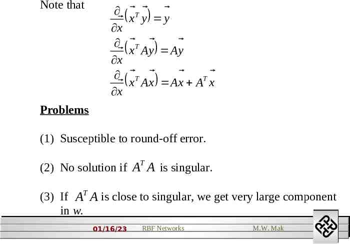
Note that T x y y x T x Ay Ay x T T x Ax Ax A x x Problems (1) Susceptible to round-off error. T (2) No solution if A A is singular. (3) If AT A is close to singular, we get very large component in w. 01/16/23 RBF Networks M.W. Mak 1

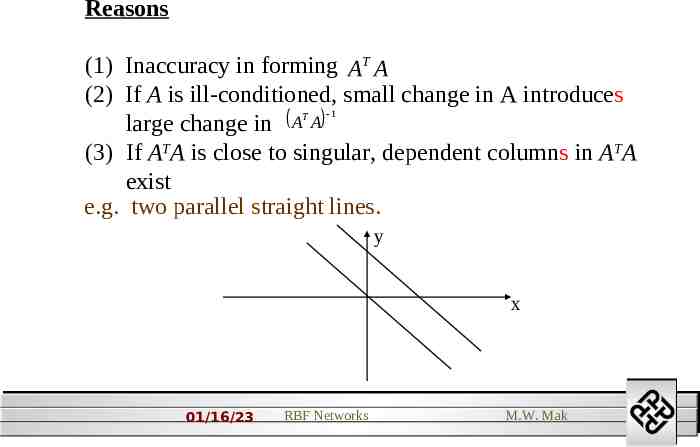
Reasons (1) Inaccuracy in forming AT A (2) If A is ill-conditioned, small change in A introduces 1 T A A large change in (3) If ATA is close to singular, dependent columns in ATA exist e.g. two parallel straight lines. y x 01/16/23 RBF Networks M.W. Mak 1

singular matrix : 1 2 x 0 2 4 y 1 If the lines are nearly parallel, they intersect each other at , i.e. x0 y 0 or x0 y 0 So, the magnitude of the solution becomes very large; hence overflow will occur. The effect of the large components can be cancelled out if the machine precision is infinite. 01/16/23 RBF Networks M.W. Mak 1

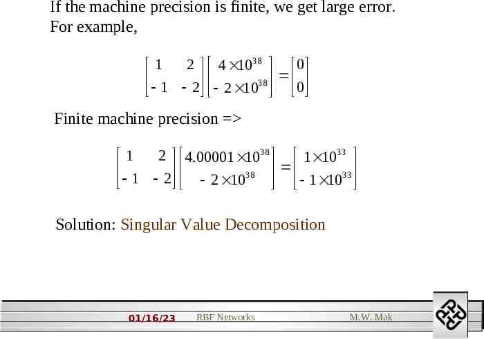
If the machine precision is finite, we get large error. For example, 2 4 1038 0 1 1 2 38 2 10 0 Finite machine precision 2 4.00001 1038 1 1033 1 1 2 38 33 2 10 1 10 Solution: Singular Value Decomposition 01/16/23 RBF Networks M.W. Mak 1

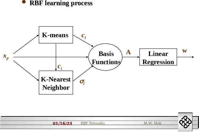
RBF learning process K-means ci A Basis Functions xp ci K-Nearest Neighbor 01/16/23 Linear Regression w i RBF Networks M.W. Mak 1

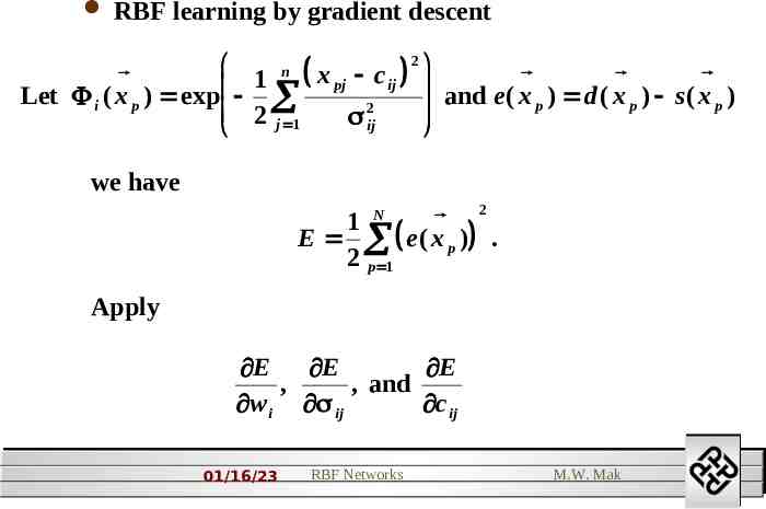
RBF learning by gradient descent 2 n x pj c ij 1 and e ( x ) d ( x ) s( x ) Let i ( x p ) exp p p p 2 2 j 1 ij we have N 2 1 E e ( x p ) . 2 p 1 Apply E E E , , and w i ij c ij 01/16/23 RBF Networks M.W. Mak 1

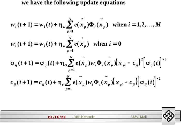
we have the following update equations N w i ( t 1) w i ( t ) w e ( x p ) i ( x p ) when i 1,2, , M p 1 N w i ( t 1) w i ( t ) w e ( x p ) when i 0 p 1 N 2 ij ( t 1) ij ( t ) e ( x p )w i i ( x p ) x pj c ij ij ( t ) p 1 N c ij ( t 1) c ij ( t ) c e ( x p )w i i ( x p ) x pj c ij ij ( t ) p 1 01/16/23 RBF Networks M.W. Mak 3 2 1

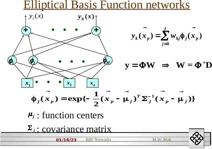
Elliptical Basis Function networks y1 ( x ) yK ( x ) J yk ( x p ) w kj j ( x p ) j 0 1 M 2 x1 x2 y W W D xn 1 j ( x p ) exp{ ( x p j )T j 1 ( x p j )} 2 : function centers j : covariance matrix j 01/16/23 RBF Networks M.W. Mak 2

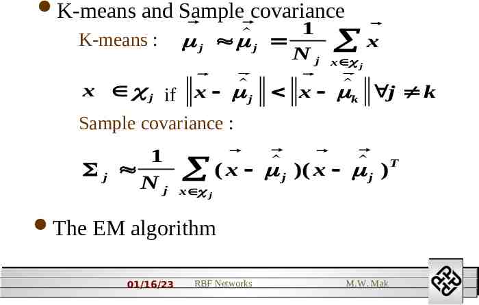
K-means and Sample covariance 1 K-means : j j x N j x j x j if x j x k j k Sample covariance : 1 j Nj )T ( x )( x j j x j The EM algorithm 01/16/23 RBF Networks M.W. Mak 2

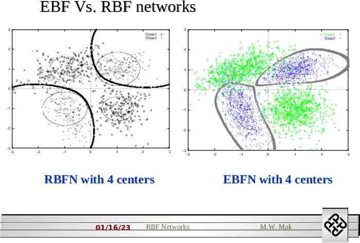
EBF Vs. RBF networks 3 3 Class 1 Class 2 Class 1 Class 2 2 2 1 1 0 0 -1 -1 -2 -3 -2 -3 -2 -1 0 1 2 3 -3 -3 RBFN with 4 centers 01/16/23 RBF Networks -2 -1 0 1 2 3 EBFN with 4 centers M.W. Mak 2

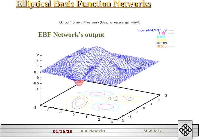
Elliptical Basis Function Networks Out put 1 of an EBF net work (bias, no rescale, gamma 1) 'nxor.ebf 4.Y.N.1.dat ' 1.43 0.948 0.463 -0.0209 -0.505 EBF Network’s output 2 1.5 1 0.5 0 -0.5 -1 3 2 1 -3 -2 0 -1 01/16/23 0 -1 1 -2 2 RBF Networks 3 -3 M.W. Mak 2

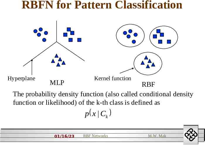
RBFN for Pattern Classification Hyperplane MLP Kernel function RBF The probability density function (also called conditional density function or likelihood) of the k-th class is defined as p x Ck 01/16/23 RBF Networks M.W. Mak 2

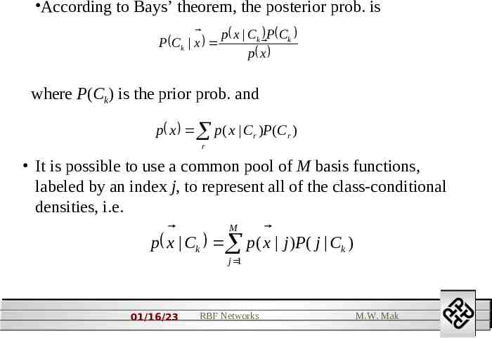
According to Bays’ theorem, the posterior prob. is p x Ck P Ck P Ck x p x where P(Ck) is the prior prob. and p x p ( x Cr )P(Cr ) r It is possible to use a common pool of M basis functions, labeled by an index j, to represent all of the class-conditional densities, i.e. M p x Ck p ( x j )P( j Ck ) j 1 01/16/23 RBF Networks M.W. Mak 2

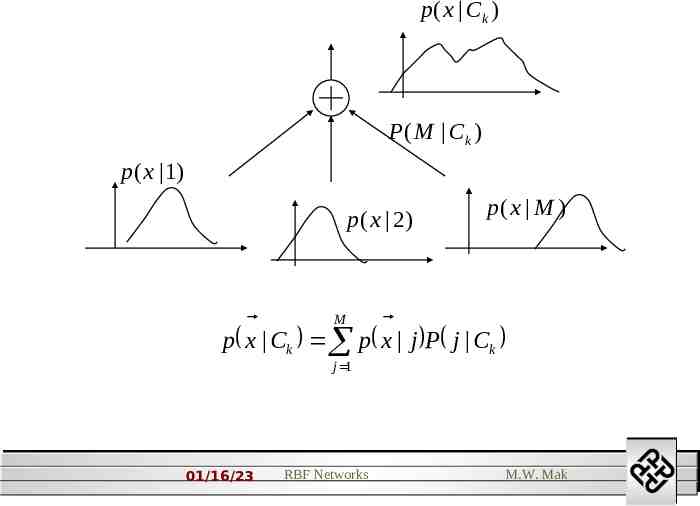
p ( x Ck ) P ( M Ck ) p(x 1) p(x 2) p( x M ) M p x Ck p x j P j Ck j 1 01/16/23 RBF Networks M.W. Mak 2

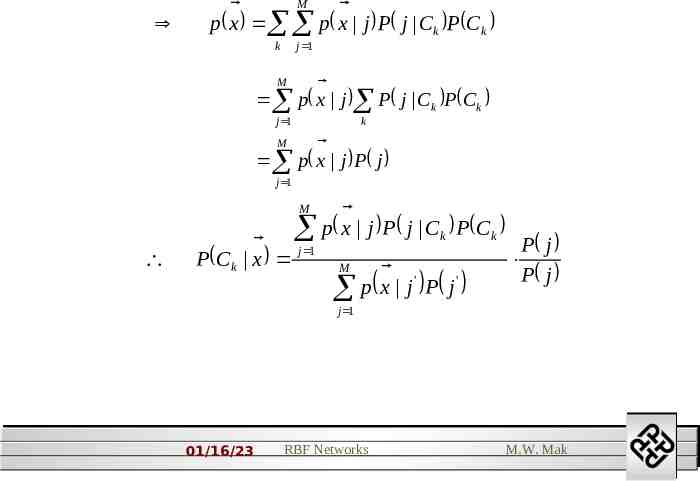
M p x p x j P j Ck P Ck k j 1 M p x j P j C k P C k j 1 k M p x j P j j 1 M p x j P j C k P Ck P Ck x j 1 M ' ' p x j P j P j P j j 1 01/16/23 RBF Networks M.W. Mak 2

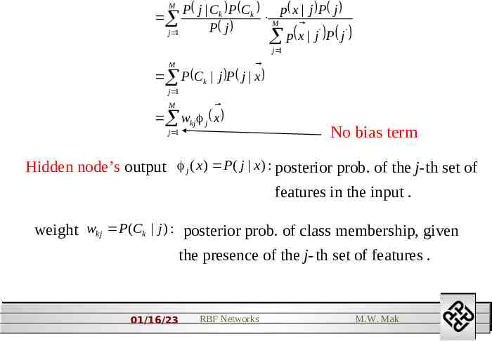
P j Ck P Ck p x j P j M ' P j j 1 p x j P j ' M j 1 M P C k j P j x j 1 M wkj j x j 1 No bias term Hidden node’s output j ( x ) P( j x ) : posterior prob. of the j-th set of features in the input . weight wkj P(Ck j ) : posterior prob. of class membership, given the presence of the j- th set of features . 01/16/23 RBF Networks M.W. Mak 2

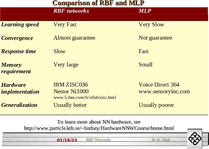
Comparison of RBF and MLP RBF networks MLP Learning speed Very Fast Very Slow Convergence Almost guarantee Not guarantee Response time Slow Fast Memory requirement Very large Small Hardware implementation IBM ZISC036 Nestor Ni1000 Voice Direct 364 www.sensoryinc.com www-5.ibm.com/fr/cdlab/zisc.html Generalization Usually better Usually poorer To learn more about NN hardware, see http://www.particle.kth.se/ lindsey/HardwareNNWCourse/home.html 01/16/23 RBF Networks M.W. Mak 2