NP and NPCompleteness Bryan Pearsaul
20 Slides188.50 KB
NP and NPCompleteness Bryan Pearsaul
Outline Decision and Optimization Problems P and NP Polynomial-Time Reducibility NP-Hardness and NP-Completeness Examples: TSP, Circuit-SAT, Knapsack Polynomial-Time Approximation Schemes
Outline Backtracking Branch-and-Bound Summary References
Decision and Optimization Problems Decision Problem: computational problem with intended output of “yes” or “no”, 1 or 0 Optimization Problem: computational problem where we try to maximize or minimize some value Introduce parameter k and ask if the optimal value for the problem is a most or at least k. Turn optimization into decision
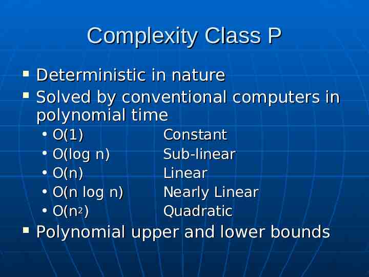
Complexity Class P Deterministic in nature Solved by conventional computers in polynomial time O(1) O(log n) O(n) O(n log n) O(n2) Constant Sub-linear Linear Nearly Linear Quadratic Polynomial upper and lower bounds
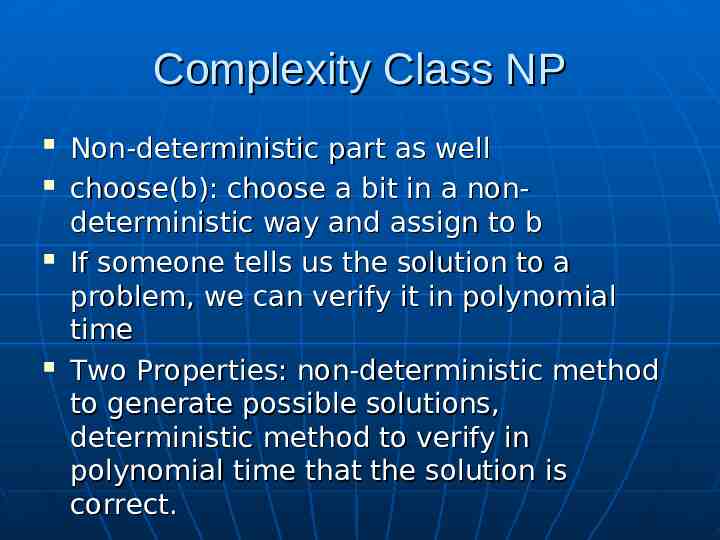
Complexity Class NP Non-deterministic part as well choose(b): choose a bit in a nondeterministic way and assign to b If someone tells us the solution to a problem, we can verify it in polynomial time Two Properties: non-deterministic method to generate possible solutions, deterministic method to verify in polynomial time that the solution is correct.
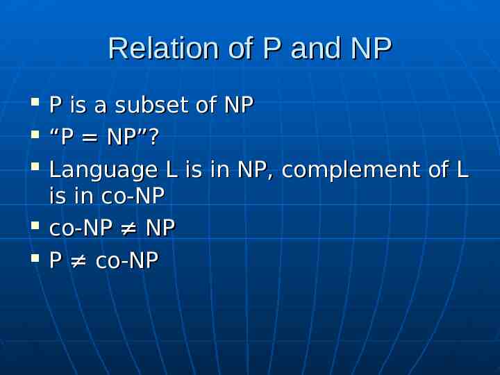
Relation of P and NP P is a subset of NP “P NP”? Language L is in NP, complement of L is in co-NP co-NP NP P co-NP
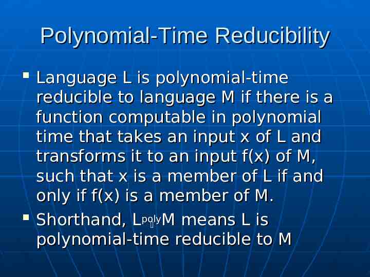
Polynomial-Time Reducibility Language L is polynomial-time reducible to language M if there is a function computable in polynomial time that takes an input x of L and transforms it to an input f(x) of M, such that x is a member of L if and only if f(x) is a member of M. Shorthand, Lpoly M means L is polynomial-time reducible to M
NP-Hard and NP-Complete Language M is NP-hard if every other language L in NP is polynomial-time reducible to M For every L that is a member of NP, Lpoly M If language M is NP-hard and also in the class of NP itself, then M is NPcomplete
NP-Hard and NP-Complete Restriction: A known NP-complete problem M is actually just a special case of L Local replacement: reduce a known NPcomplete problem M to L by dividing instances of M and L into “basic units” then showing each unit of M can be converted to a unit of L Component design: reduce a known NPcomplete problem M to L by building components for an instance of L that enforce important structural functions for instances of M.
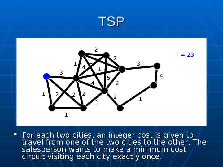
TSP 2 1 3 4 2 1 1 5 4 1 2 2 2 1 i 23 3 4 2 2 1 1 For each two cities, an integer cost is given to travel from one of the two cities to the other. The salesperson wants to make a minimum cost circuit visiting each city exactly once.
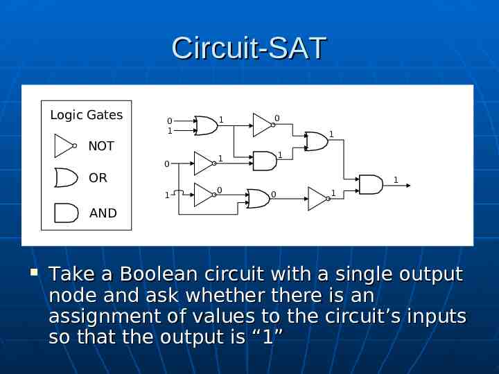
Circuit-SAT Logic Gates 0 1 NOT 0 1 0 1 1 1 OR 1 1 0 0 1 AND Take a Boolean circuit with a single output node and ask whether there is an assignment of values to the circuit’s inputs so that the output is “1”
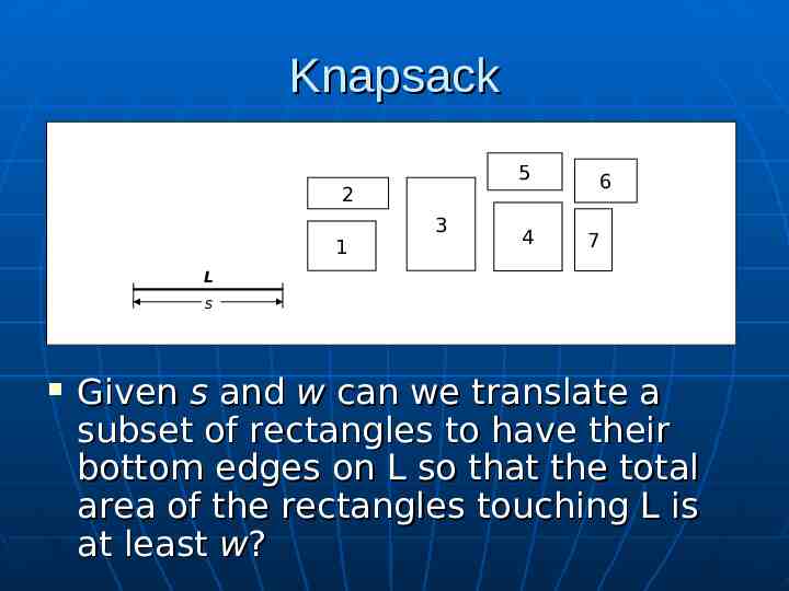
Knapsack 5 2 1 3 4 6 7 L s Given s and w can we translate a subset of rectangles to have their bottom edges on L so that the total area of the rectangles touching L is at least w?
PTAS Polynomial-Time Approximation Schemes Much faster, but not guaranteed to find the best solution Come as close to the optimum value as possible in a reasonable amount of time Take advantage of rescalability property of some hard problems
Backtracking Effective for decision problems Systematically traverse through possible paths to locate solutions or dead ends At the end of the path, algorithm is left with (x, y) pair. x is remaining subproblem, y is set of choices made to get to x Initially (x, Ø) passed to algorithm
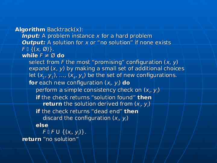
Algorithm Backtrack(x): Input: A problem instance x for a hard problem Output: A solution for x or “no solution” if none exists F {(x, Ø)}. while F Ø do select from F the most “promising” configuration (x, y) expand (x, y) by making a small set of additional choices let (x1, y1), , (xk, yk) be the set of new configurations. for each new configuration (xi, yi) do perform a simple consistency check on (xi, yi) if the check returns “solution found” then return the solution derived from (xi, yi) if the check returns “dead end” then discard the configuration (xi, yi) else F F U {(xi, yi)}. return “no solution”
Branch-and-Bound Effective for optimization problems Extended Backtracking Algorithm Instead of stopping once a single solution is found, continue searching until the best solution is found Has a scoring mechanism to choose most promising configuration in each iteration
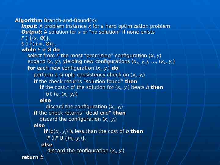
Algorithm Branch-and-Bound(x): Input: A problem instance x for a hard optimization problem Output: A solution for x or “no solution” if none exists F {(x, Ø)}. b {( , Ø)}. while F Ø do select from F the most “promising” configuration ( x, y) expand (x, y), yielding new configurations (x1, y1), , (xk, yk) for each new configuration (xi, yi) do perform a simple consistency check on ( xi, yi) if the check returns “solution found” then if the cost c of the solution for (xi, yi) beats b then b (c, (xi, yi)) else discard the configuration (xi, yi) if the check returns “dead end” then discard the configuration (xi, yi) else if lb(xi, yi) is less than the cost of b then F F U {(xi, yi)}. else discard the configuration (xi, yi) return b
Summary Decision and Optimization Problems P and NP Polynomial-Time Reducibility NP-Hardness and NP-Completeness TSP, Circuit-SAT, Knapsack PTAS Backtracking/Branch-and-Bound
References A.K. Dewdney, The New Turning Omnibus, pp. 276-281, 357-362, Henry Holt and Company, 2001. Goodrich & Tamassia, Algorithm Design, pp. 592-637, John Wiley & Sons, Inc., 2002.