ANOVA: Analysis of Variation Math 143 Lecture R. Pruim


30 Slides134.50 KB
ANOVA: Analysis of Variation Math 143 Lecture R. Pruim
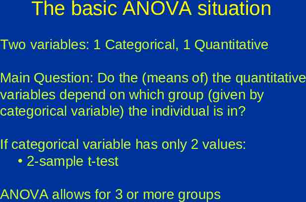
The basic ANOVA situation Two variables: 1 Categorical, 1 Quantitative Main Question: Do the (means of) the quantitative variables depend on which group (given by categorical variable) the individual is in? If categorical variable has only 2 values: 2-sample t-test ANOVA allows for 3 or more groups
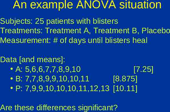
An example ANOVA situation Subjects: 25 patients with blisters Treatments: Treatment A, Treatment B, Placebo Measurement: # of days until blisters heal Data [and means]: A: 5,6,6,7,7,8,9,10 [7.25] B: 7,7,8,9,9,10,10,11 [8.875] P: 7,9,9,10,10,10,11,12,13 [10.11] Are these differences significant?
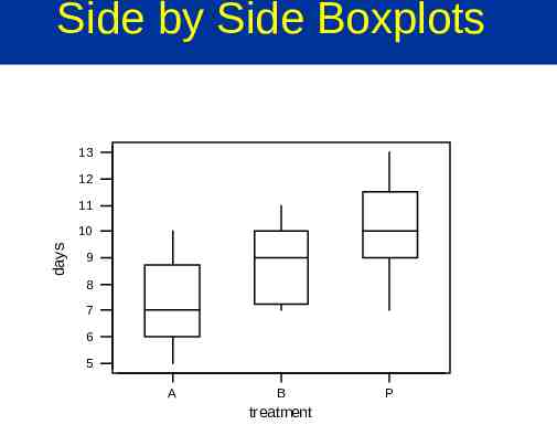
Informal Investigation Graphical investigation: side-by-side box plots multiple histograms Whether the differences between the groups are significant depends on the difference in the means the standard deviations of each group the sample sizes ANOVA determines P-value from the F statistic
Side by Side Boxplots 13 12 11 days 10 9 8 7 6 5 A B treatment P
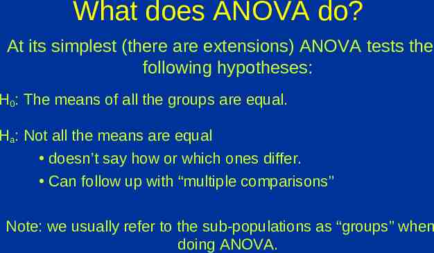
What does ANOVA do? At its simplest (there are extensions) ANOVA tests the following hypotheses: H0: The means of all the groups are equal. Ha: Not all the means are equal doesn’t say how or which ones differ. Can follow up with “multiple comparisons” Note: we usually refer to the sub-populations as “groups” when doing ANOVA.
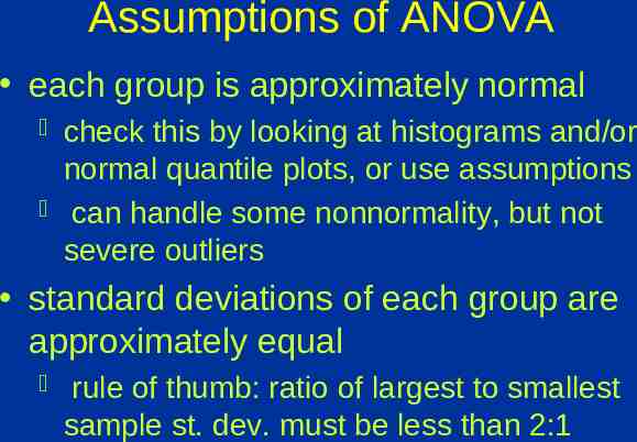
Assumptions of ANOVA each group is approximately normal check this by looking at histograms and/or normal quantile plots, or use assumptions can handle some nonnormality, but not severe outliers standard deviations of each group are approximately equal rule of thumb: ratio of largest to smallest sample st. dev. must be less than 2:1
Normality Check We should check for normality using: assumptions about population histograms for each group normal quantile plot for each group With such small data sets, there really isn’t a really good way to check normality from data, but we make the common assumption that physical measurements of people tend to be normally distributed.
Standard Deviation Check Variable days treatment A B P N 8 8 9 Mean 7.250 8.875 10.111 Median 7.000 9.000 10.000 StDev 1.669 1.458 1.764 Compare largest and smallest standard deviations: largest: 1.764 smallest: 1.458 1.458 x 2 2.916 1.764 Note: variance ratio of 4:1 is equivalent.
Notation for ANOVA n number of individuals all together I number of groups x mean for entire data set is Group i has ni # of individuals in group i xij value for individual j in group i x i mean for group i si standard deviation for group i
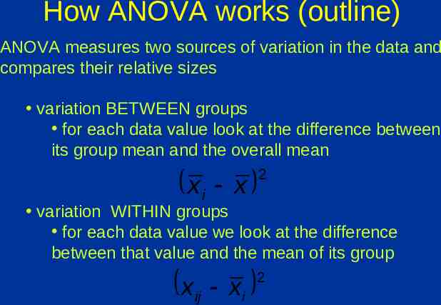
How ANOVA works (outline) ANOVA measures two sources of variation in the data and compares their relative sizes variation BETWEEN groups for each data value look at the difference between its group mean and the overall mean xi x 2 variation WITHIN groups for each data value we look at the difference between that value and the mean of its group x ij xi 2
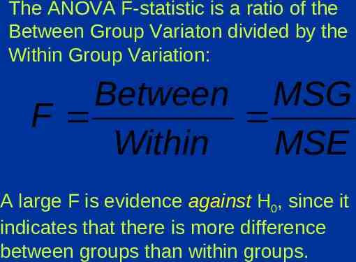
The ANOVA F-statistic is a ratio of the Between Group Variaton divided by the Within Group Variation: Between MSG F Within MSE A large F is evidence against H0, since it indicates that there is more difference between groups than within groups.
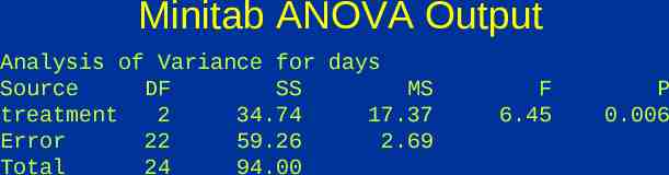
Minitab ANOVA Output Analysis of Variance for days Source DF SS MS treatment 2 34.74 17.37 Error 22 59.26 2.69 Total 24 94.00 F 6.45 P 0.006
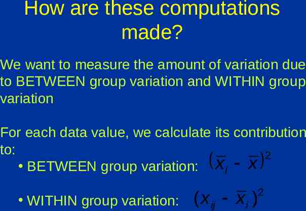
How are these computations made? We want to measure the amount of variation due to BETWEEN group variation and WITHIN group variation For each data value, we calculate its contribution to: 2 BETWEEN group variation: x i x WITHIN group variation: ( x ij x i ) 2
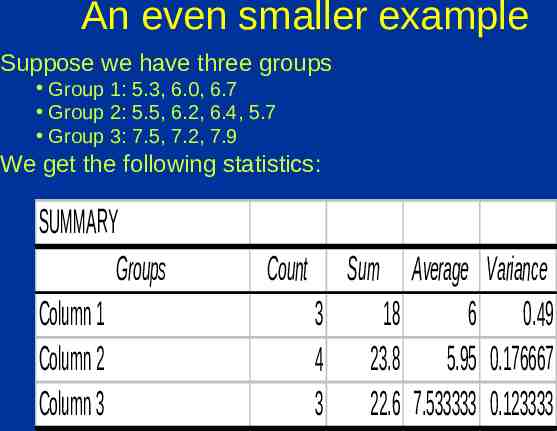
An even smaller example Suppose we have three groups Group 1: 5.3, 6.0, 6.7 Group 2: 5.5, 6.2, 6.4, 5.7 Group 3: 7.5, 7.2, 7.9 We get the following statistics: SUMMARY Groups Column 1 Column 2 Column 3 Count Sum Average Variance 3 18 6 0.49 4 23.8 5.95 0.176667 3 22.6 7.533333 0.123333
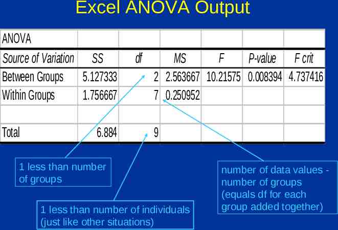
Excel ANOVA Output ANOVA Source of Variation SS Between Groups 5.127333 Within Groups 1.756667 Total 6.884 df MS F P-value F crit 2 2.563667 10.21575 0.008394 4.737416 7 0.250952 9 1 less than number of groups 1 less than number of individuals (just like other situations) number of data values number of groups (equals df for each group added together)
Computing ANOVA F statistic data group 5.3 1 6.0 1 6.7 1 5.5 2 6.2 2 6.4 2 5.7 2 7.5 3 7.2 3 7.9 3 TOTAL TOTAL/df group mean 6.00 6.00 6.00 5.95 5.95 5.95 5.95 7.53 7.53 7.53 WITHIN difference: data - group mean plain squared -0.70 0.490 0.00 0.000 0.70 0.490 -0.45 0.203 0.25 0.063 0.45 0.203 -0.25 0.063 -0.03 0.001 -0.33 0.109 0.37 0.137 1.757 0.25095714 overall mean: 6.44 BETWEEN difference group mean - overall mean plain squared -0.4 0.194 -0.4 0.194 -0.4 0.194 -0.5 0.240 -0.5 0.240 -0.5 0.240 -0.5 0.240 1.1 1.188 1.1 1.188 1.1 1.188 5.106 2.55275 F 2.5528/0.25025 10.21575
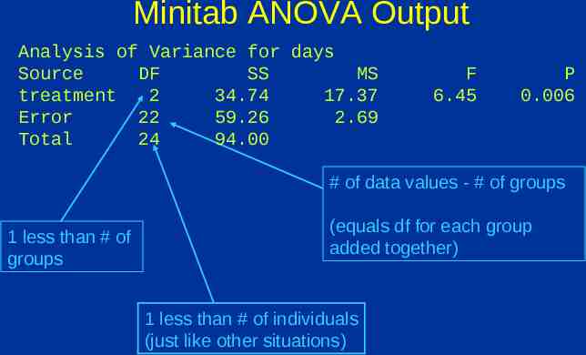
Minitab ANOVA Output Analysis of Variance for days Source DF SS MS treatment 2 34.74 17.37 Error 22 59.26 2.69 Total 24 94.00 F 6.45 P 0.006 # of data values - # of groups 1 less than # of groups (equals df for each group added together) 1 less than # of individuals (just like other situations)
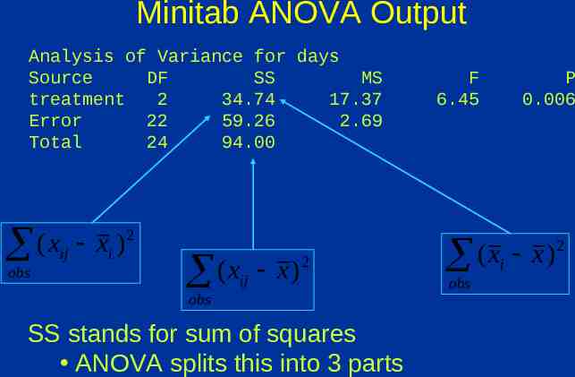
Minitab ANOVA Output Analysis of Variance for days Source DF SS MS treatment 2 34.74 17.37 Error 22 59.26 2.69 Total 24 94.00 (x ij obs xi ) 2 ( xij x ) 2 obs SS stands for sum of squares ANOVA splits this into 3 parts F 6.45 P 0.006 (x x) i obs 2
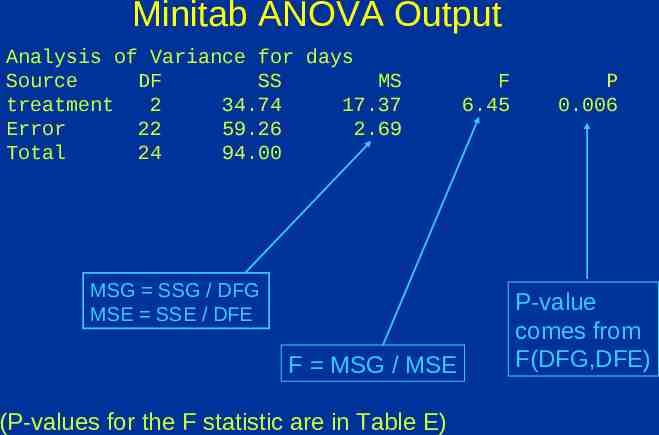
Minitab ANOVA Output Analysis of Variance for days Source DF SS MS treatment 2 34.74 17.37 Error 22 59.26 2.69 Total 24 94.00 MSG SSG / DFG MSE SSE / DFE F MSG / MSE (P-values for the F statistic are in Table E) F 6.45 P 0.006 P-value comes from F(DFG,DFE)
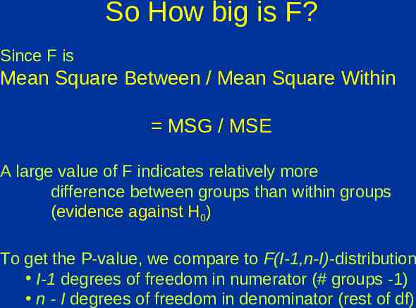
So How big is F? Since F is Mean Square Between / Mean Square Within MSG / MSE A large value of F indicates relatively more difference between groups than within groups (evidence against H0) To get the P-value, we compare to F(I-1,n-I)-distribution I-1 degrees of freedom in numerator (# groups -1) n - I degrees of freedom in denominator (rest of df)
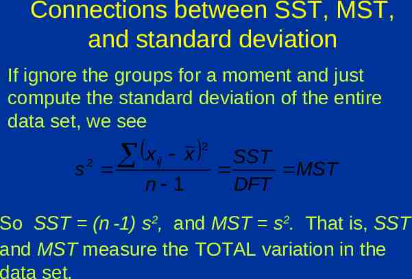
Connections between SST, MST, and standard deviation If ignore the groups for a moment and just compute the standard deviation of the entire data set, we see s 2 x ij x n 1 2 SST MST DFT So SST (n -1) s2, and MST s2. That is, SST and MST measure the TOTAL variation in the data set.
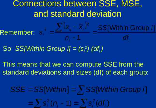
Connections between SSE, MSE, and standard deviation Remember: si 2 x ij xi ni 1 2 SS [ Within Group i ] dfi So SS[Within Group i] (si2) (dfi ) This means that we can compute SSE from the standard deviations and sizes (df) of each group: SSE SS[Within ] SS[Within Group i ] si2 (ni 1) si2 (dfi )
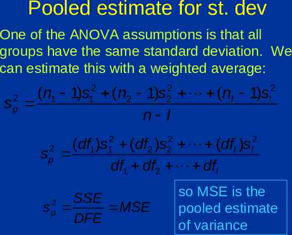
Pooled estimate for st. dev One of the ANOVA assumptions is that all groups have the same standard deviation. We can estimate this with a weighted average: 2 2 2 ( n 1 ) s ( n 1 ) s ( n 1 ) s 1 2 2 I I s p2 1 n I 2 2 2 ( df ) s ( df ) s ( df ) s 2 2 I I s p2 1 1 df1 df2 dfI SSE 2 sp MSE DFE so MSE is the pooled estimate of variance
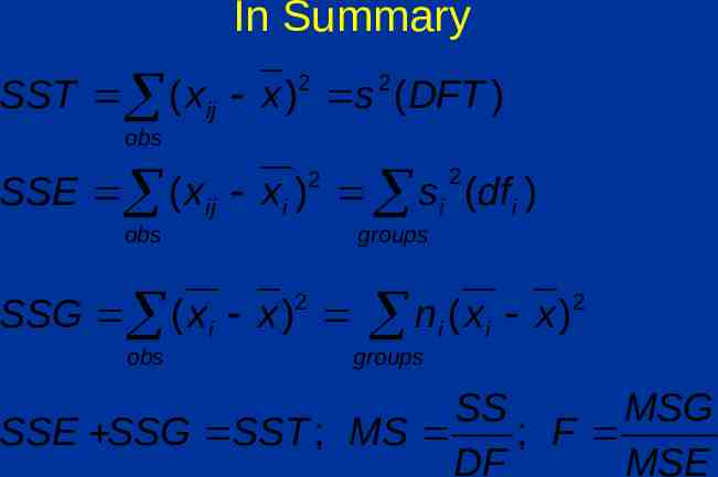
In Summary 2 2 SST ( x ij x ) s (DFT ) obs 2 2 SSE ( x ij x i ) si (dfi ) obs groups 2 SSG ( x i x ) obs n (x i i x) 2 groups SS MSG SSE SSG SST ; MS ; F DF MSE
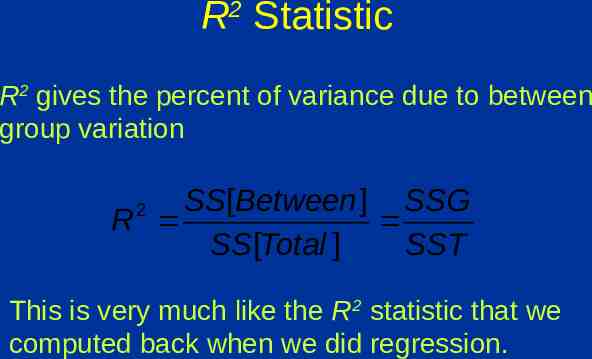
R Statistic 2 R2 gives the percent of variance due to between group variation SS[Between ] SSG R SS[Total ] SST 2 This is very much like the R2 statistic that we computed back when we did regression.
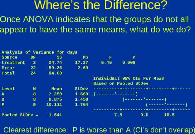
Where’s the Difference? Once ANOVA indicates that the groups do not all appear to have the same means, what do we do? Analysis of Variance for days Source DF SS MS treatment 2 34.74 17.37 Error 22 59.26 2.69 Total 24 94.00 Level A B P N 8 8 9 Pooled StDev Mean 7.250 8.875 10.111 1.641 StDev 1.669 1.458 1.764 F 6.45 P 0.006 Individual 95% CIs For Mean Based on Pooled StDev ---------- --------- --------- -----(-------*-------) (-------*-------) (------*-------) ---------- --------- --------- -----7.5 9.0 10.5 Clearest difference: P is worse than A (CI’s don’t overlap)
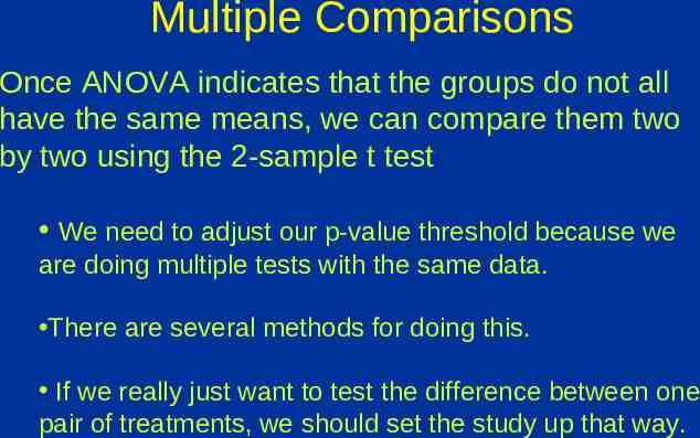
Multiple Comparisons Once ANOVA indicates that the groups do not all have the same means, we can compare them two by two using the 2-sample t test We need to adjust our p-value threshold because we are doing multiple tests with the same data. There are several methods for doing this. If we really just want to test the difference between one pair of treatments, we should set the study up that way.
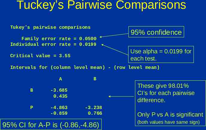
Tuckey’s Pairwise Comparisons Tukey's pairwise comparisons Family error rate 0.0500 Individual error rate 0.0199 95% confidence Use alpha 0.0199 for each test. Critical value 3.55 Intervals for (column level mean) - (row level mean) A B -3.685 0.435 P -4.863 -0.859 B These give 98.01% CI’s for each pairwise difference. -3.238 0.766 95% CI for A-P is (-0.86,-4.86) Only P vs A is significant (both values have same sign)
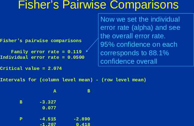
Fisher’s Pairwise Comparisons Now we set the individual error rate (alpha) and see the overall error rate. 95% confidence on each corresponds to 88.1% confidence overall Fisher's pairwise comparisons Family error rate 0.119 Individual error rate 0.0500 Critical value 2.074 Intervals for (column level mean) - (row level mean) A B -3.327 0.077 P -4.515 -1.207 B -2.890 0.418