Introduction to Neural Networks CS405


54 Slides1.45 MB
Introduction to Neural Networks CS405
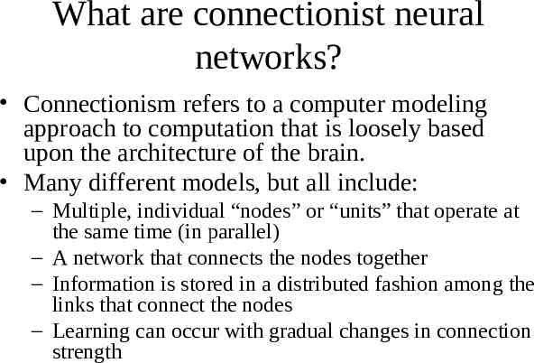
What are connectionist neural networks? Connectionism refers to a computer modeling approach to computation that is loosely based upon the architecture of the brain. Many different models, but all include: – Multiple, individual “nodes” or “units” that operate at the same time (in parallel) – A network that connects the nodes together – Information is stored in a distributed fashion among the links that connect the nodes – Learning can occur with gradual changes in connection strength
Neural Network History History traces back to the 50’s but became popular in the 80’s with work by Rumelhart, Hinton, and Mclelland – A General Framework for Parallel Distributed Processing in Parallel Distributed Processing: Explorations in the Microstructure of Cognition Peaked in the 90’s. Today: – Hundreds of variants – Less a model of the actual brain than a useful tool, but still some debate Numerous applications – Handwriting, face, speech recognition – Vehicles that drive themselves – Models of reading, sentence production, dreaming Debate for philosophers and cognitive scientists – Can human consciousness or cognitive abilities be explained by a connectionist model or does it require the manipulation of symbols?
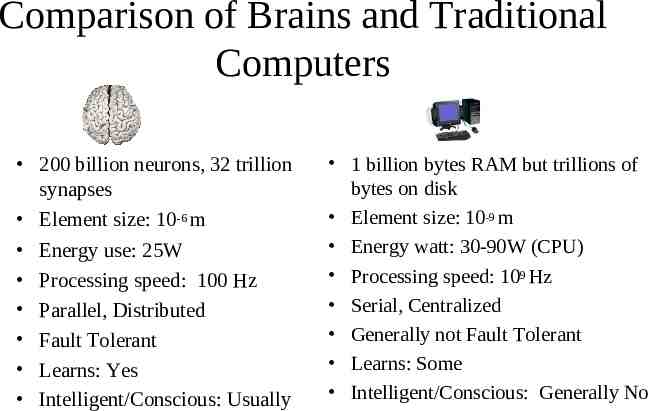
Comparison of Brains and Traditional Computers 200 billion neurons, 32 trillion synapses Element size: 10-6 m Energy use: 25W Processing speed: 100 Hz Parallel, Distributed Fault Tolerant Learns: Yes Intelligent/Conscious: Usually 1 billion bytes RAM but trillions of bytes on disk Element size: 10-9 m Energy watt: 30-90W (CPU) Processing speed: 109 Hz Serial, Centralized Generally not Fault Tolerant Learns: Some Intelligent/Conscious: Generally No
Biological Inspiration Idea : To make the computer more robust, intelligent, and learn, Let’s model our computer software (and/or hardware) after the brain “My brain: It's my second favorite organ.” - Woody Allen, from the movie Sleeper
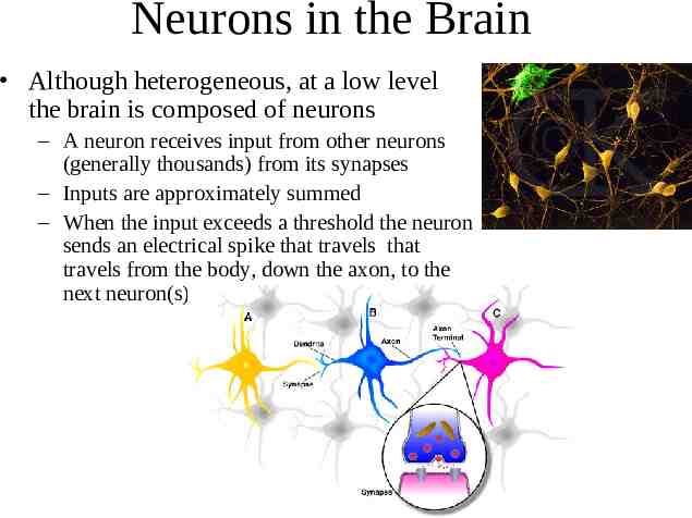
Neurons in the Brain Although heterogeneous, at a low level the brain is composed of neurons – A neuron receives input from other neurons (generally thousands) from its synapses – Inputs are approximately summed – When the input exceeds a threshold the neuron sends an electrical spike that travels that travels from the body, down the axon, to the next neuron(s)
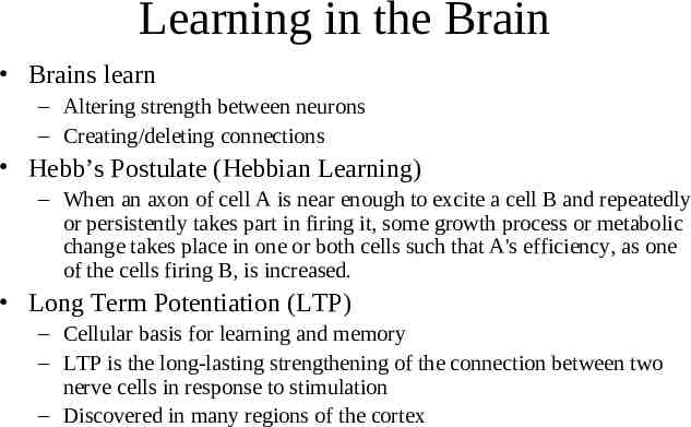
Learning in the Brain Brains learn – Altering strength between neurons – Creating/deleting connections Hebb’s Postulate (Hebbian Learning) – When an axon of cell A is near enough to excite a cell B and repeatedly or persistently takes part in firing it, some growth process or metabolic change takes place in one or both cells such that A's efficiency, as one of the cells firing B, is increased. Long Term Potentiation (LTP) – Cellular basis for learning and memory – LTP is the long-lasting strengthening of the connection between two nerve cells in response to stimulation – Discovered in many regions of the cortex
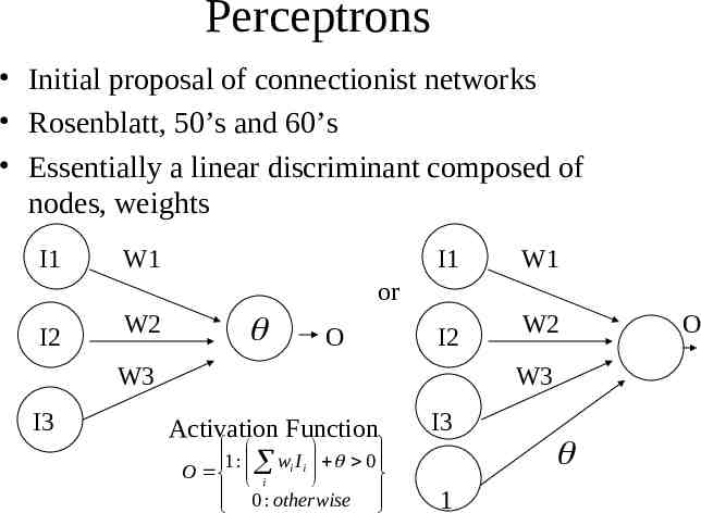
Perceptrons Initial proposal of connectionist networks Rosenblatt, 50’s and 60’s Essentially a linear discriminant composed of nodes, weights I1 W1 I1 W1 I2 W2 or I2 W2 O W3 I3 W3 Activation Function 1 : wi I i 0 O i 0 : otherwise I3 1 O
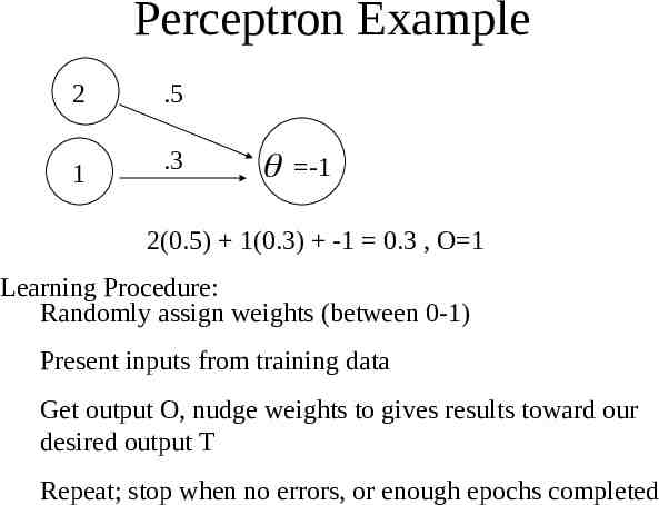
Perceptron Example 2 1 .5 .3 -1 2(0.5) 1(0.3) -1 0.3 , O 1 Learning Procedure: Randomly assign weights (between 0-1) Present inputs from training data Get output O, nudge weights to gives results toward our desired output T Repeat; stop when no errors, or enough epochs completed
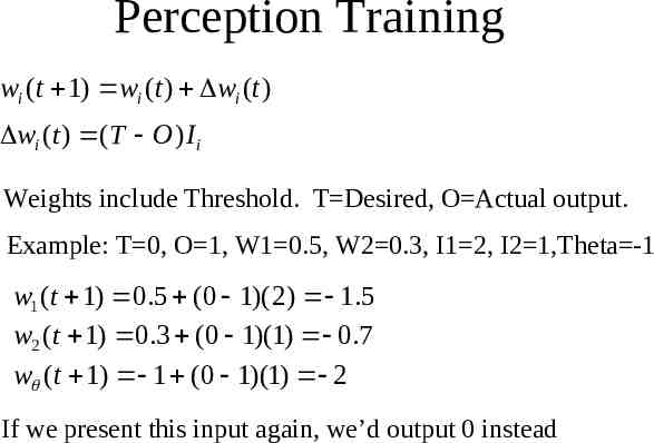
Perception Training wi (t 1) wi (t ) wi (t ) wi (t ) (T O ) I i Weights include Threshold. T Desired, O Actual output. Example: T 0, O 1, W1 0.5, W2 0.3, I1 2, I2 1,Theta -1 w1 (t 1) 0.5 (0 1)( 2) 1.5 w2 (t 1) 0.3 (0 1)(1) 0.7 w (t 1) 1 (0 1)(1) 2 If we present this input again, we’d output 0 instead
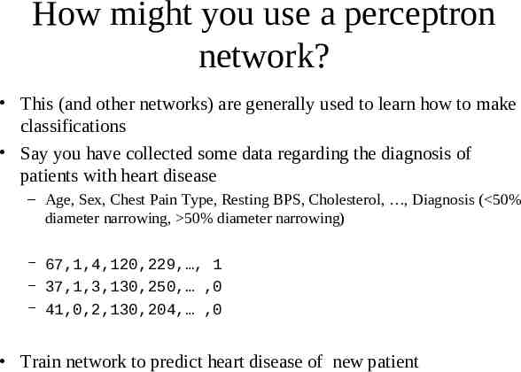
How might you use a perceptron network? This (and other networks) are generally used to learn how to make classifications Say you have collected some data regarding the diagnosis of patients with heart disease – Age, Sex, Chest Pain Type, Resting BPS, Cholesterol, , Diagnosis ( 50% diameter narrowing, 50% diameter narrowing) – 67,1,4,120,229, , 1 – 37,1,3,130,250, ,0 – 41,0,2,130,204, ,0 Train network to predict heart disease of new patient
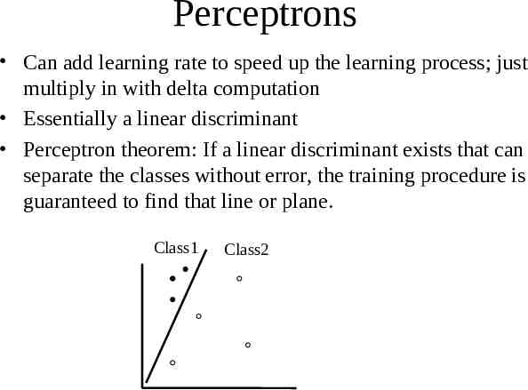
Perceptrons Can add learning rate to speed up the learning process; just multiply in with delta computation Essentially a linear discriminant Perceptron theorem: If a linear discriminant exists that can separate the classes without error, the training procedure is guaranteed to find that line or plane. Class1 Class2
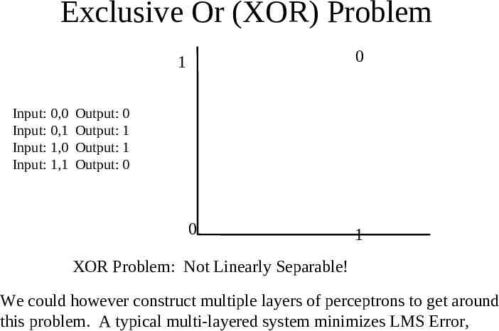
Exclusive Or (XOR) Problem 0 1 Input: 0,0 Input: 0,1 Input: 1,0 Input: 1,1 Output: 0 Output: 1 Output: 1 Output: 0 0 1 XOR Problem: Not Linearly Separable! We could however construct multiple layers of perceptrons to get around this problem. A typical multi-layered system minimizes LMS Error,
LMS Learning LMS Least Mean Square learning Systems, more general than the previous perceptron learning rule. The concept is to minimize the total error, as measured over all training examples, P. O is the raw output, as calculated by wi I i 1 2 Dis tan ce( LMS ) TP OP 2 P i E.g. if we have two patterns and T1 1, O1 0.8, T2 0, O2 0.5 then D (0.5)[(1-0.8)2 (0-0.5)2] .145 We want to minimize the LMS: C-learning rate E W(old) W(new) W
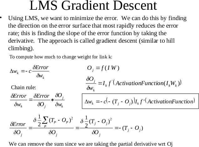
LMS Gradient Descent Using LMS, we want to minimize the error. We can do this by finding the direction on the error surface that most rapidly reduces the error rate; this is finding the slope of the error function by taking the derivative. The approach is called gradient descent (similar to hill climbing). To compute how much to change weight for link k: wk c Error wk Chain rule: Error Error O j wk O j wk Oj f (I W ) O j I k f ' ActivationFunction( I kWk ) wk wk c (T j O j ) I k f ' ActivationFunction 1 2 1 2 ( T O ) ( T O ) P P j j Error 2 P 2 (T j O j ) O j O j O j We can remove the sum since we are taking the partial derivative wrt Oj
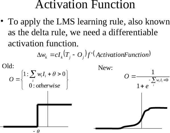
Activation Function To apply the LMS learning rule, also known as the delta rule, we need a differentiable activation function. wk cI k T j O j f ' ActivationFunction Old: 1 : wi I i 0 O i 0 : otherwise New: O 1 e 1 wi I i i
LMS vs. Limiting Threshold With the new sigmoidal function that is differentiable, we can apply the delta rule toward learning. Perceptron Method – Forced output to 0 or 1, while LMS uses the net output – Guaranteed to separate, if no error and is linearly separable Otherwise it may not converge Gradient Descent Method: – May oscillate and not converge – May converge to wrong answer – Will converge to some minimum even if the classes are not linearly separable, unlike the earlier perceptron training method
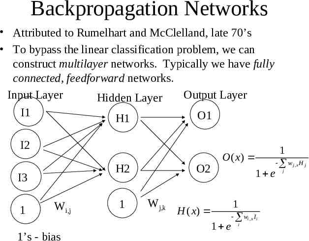
Backpropagation Networks Attributed to Rumelhart and McClelland, late 70’s To bypass the linear classification problem, we can construct multilayer networks. Typically we have fully connected, feedforward networks. Input Layer Output Layer Hidden Layer I1 O1 H1 I2 H2 I3 1 Wi,j 1’s - bias 1 O2 Wj,k O( x) 1 e 1 H ( x) wi , x I i 1 e i 1 w j,xH j j
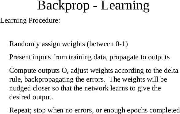
Backprop - Learning Learning Procedure: Randomly assign weights (between 0-1) Present inputs from training data, propagate to outputs Compute outputs O, adjust weights according to the delta rule, backpropagating the errors. The weights will be nudged closer so that the network learns to give the desired output. Repeat; stop when no errors, or enough epochs completed
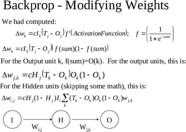
Backprop - Modifying Weights We had computed: wk cI k T j O j f ' ActivationFunction ; 1 f sum 1 e wk cI k T j O j f ( sum)(1 f ( sum) For the Output unit k, f(sum) O(k). For the output units, this is: w j ,k cH j Tk Ok Ok (1 Ok ) For the Hidden units (skipping some math), this is: wi , j cH j (1 H j ) I i (Tk Ok )Ok (1 Ok )w j ,k k I Wi,j H Wj,k O
Backprop Very powerful - can learn any function, given enough hidden units! With enough hidden units, we can generate any function. Have the same problems of Generalization vs. Memorization. With too many units, we will tend to memorize the input and not generalize well. Some schemes exist to “prune” the neural network. Networks require extensive training, many parameters to fiddle with. Can be extremely slow to train. May also fall into local minima. Inherently parallel algorithm, ideal for multiprocessor hardware. Despite the cons, a very powerful algorithm that has seen widespread successful deployment.
Backprop Demo QwikNet – Learning XOR, Sin/Cos functions
Unsupervised Learning We just discussed a form of supervised learning – A “teacher” tells the network what the correct output is based on the input until the network learns the target concept We can also train networks where there is no teacher. This is called unsupervised learning. The network learns a prototype based on the distribution of patterns in the training data. Such networks allow us to: – Discover underlying structure of the data – Encode or compress the data – Transform the data
Unsupervised Learning – Hopfield Networks A Hopfield network is a type of contentaddressable memory – Non-linear system with attractor points that represent concepts – Given a fuzzy input the system converges to the nearest attractor Possibility to have “spurious” attractors that is a blend of multiple stored patterns Also possible to have chaotic patterns that never converge
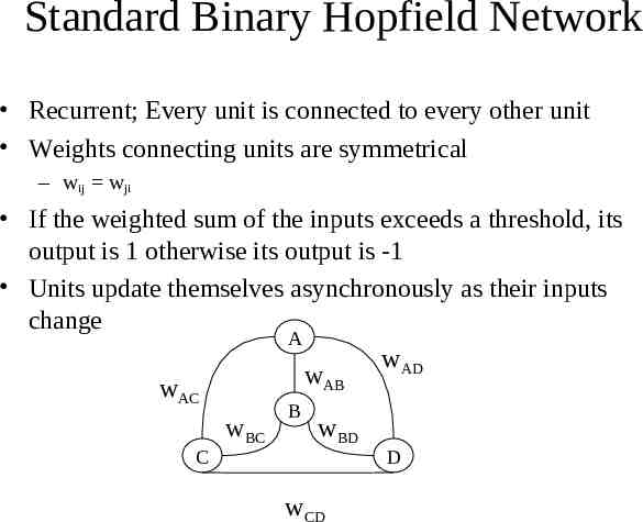
Standard Binary Hopfield Network Recurrent; Every unit is connected to every other unit Weights connecting units are symmetrical – wij wji If the weighted sum of the inputs exceeds a threshold, its output is 1 otherwise its output is -1 Units update themselves asynchronously as their inputs change A wAD w AB wAC C wBC B wBD wCD D
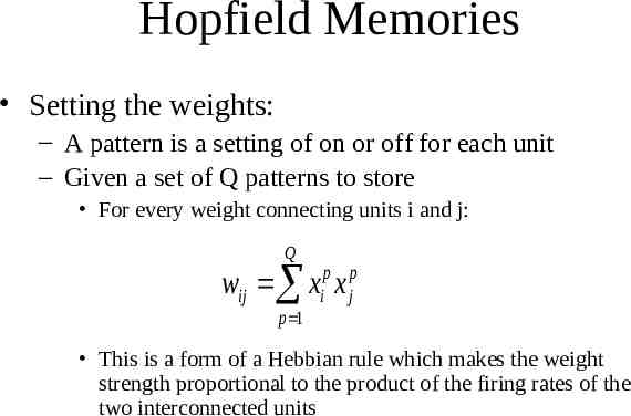
Hopfield Memories Setting the weights: – A pattern is a setting of on or off for each unit – Given a set of Q patterns to store For every weight connecting units i and j: Q wij xip x jp p 1 This is a form of a Hebbian rule which makes the weight strength proportional to the product of the firing rates of the two interconnected units
Hopfield Network Demo http://www.cbu.edu/ pong/ai/hopfield/ hopfieldapplet.html Properties – Settles into a minimal energy state – Storage capacity low, only 13% of number of units – Can retrieve information even in the presence of noisy data, similar to associative memory of humans
Unsupervised Learning – Self Organizing Maps Self-organizing maps (SOMs) are a data visualization technique invented by Professor Teuvo Kohonen – Also called Kohonen Networks, Competitive Learning, Winner-Take-All Learning – Generally reduces the dimensions of data through the use of self-organizing neural networks – Useful for data visualization; humans cannot visualize high dimensional data so this is often a useful technique to make sense of large data sets
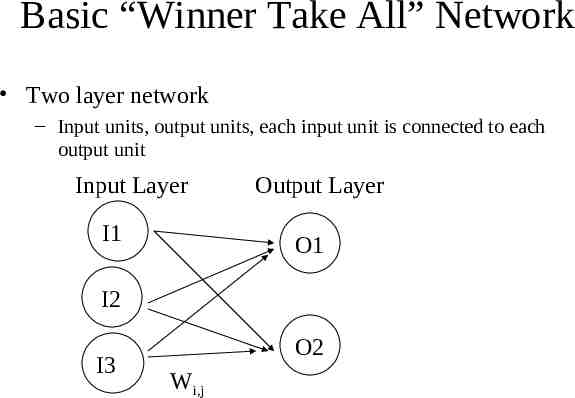
Basic “Winner Take All” Network Two layer network – Input units, output units, each input unit is connected to each output unit Input Layer I1 Output Layer O1 I2 I3 O2 Wi,j
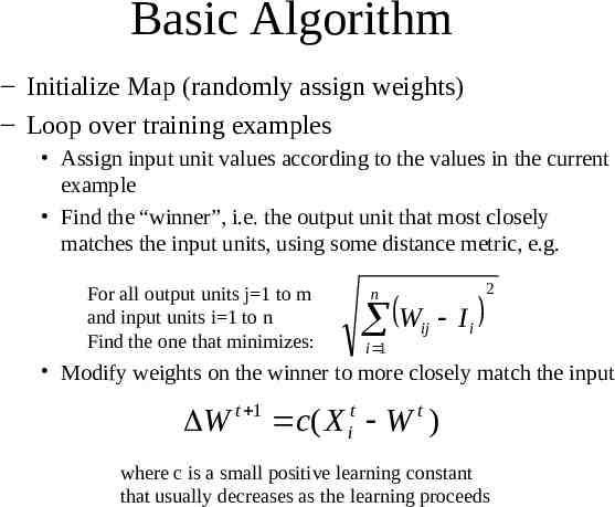
Basic Algorithm – Initialize Map (randomly assign weights) – Loop over training examples Assign input unit values according to the values in the current example Find the “winner”, i.e. the output unit that most closely matches the input units, using some distance metric, e.g. For all output units j 1 to m and input units i 1 to n Find the one that minimizes: n W ij Ii 2 i 1 Modify weights on the winner to more closely match the input W t 1 c( X it W t ) where c is a small positive learning constant that usually decreases as the learning proceeds
Result of Algorithm Initially, some output nodes will randomly be a little closer to some particular type of input These nodes become “winners” and the weights move them even closer to the inputs Over time nodes in the output become representative prototypes for examples in the input Note there is no supervised training here Classification: – Given new input, the class is the output node that is the winner
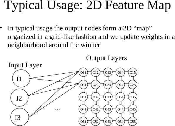
Typical Usage: 2D Feature Map In typical usage the output nodes form a 2D “map” organized in a grid-like fashion and we update weights in a neighborhood around the winner Output Layers Input Layer O11 O12 O13 O14 O15 O21 O22 O23 O24 O25 O31 O32 O33 O34 O35 O41 O42 O43 O44 O45 O51 O52 O53 O54 O55 I1 I2 I3
Modified Algorithm – Initialize Map (randomly assign weights) – Loop over training examples Assign input unit values according to the values in the current example Find the “winner”, i.e. the output unit that most closely matches the input units, using some distance metric, e.g. Modify weights on the winner to more closely match the input Modify weights in a neighborhood around the winner so the neighbors on the 2D map also become closer to the input – Over time this will tend to cluster similar items closer on the map
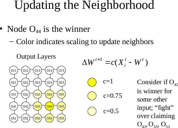
Updating the Neighborhood Node O44 is the winner – Color indicates scaling to update neighbors Output Layers W t 1 c( X it W t ) O11 O12 O13 O14 O15 O21 O22 O23 O24 O25 c 1 O31 O32 O33 O34 O35 c 0.75 O41 O42 O43 O44 O45 O51 O52 O53 O54 O55 c 0.5 Consider if O42 is winner for some other input; “fight” over claiming O43, O33, O53
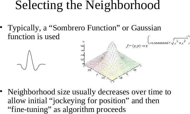
Selecting the Neighborhood Typically, a “Sombrero Function” or Gaussian function is used Neighborhood size usually decreases over time to allow initial “jockeying for position” and then “fine-tuning” as algorithm proceeds
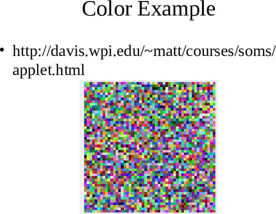
Color Example http://davis.wpi.edu/ matt/courses/soms/ applet.html
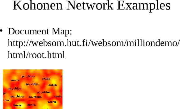
Kohonen Network Examples Document Map: http://websom.hut.fi/websom/milliondemo/ html/root.html
Poverty Map http://www.cis.hut.fi/ research/som-research/ worldmap.html
SOM for Classification A generated map can also be used for classification Human can assign a class to a data point, or use the strongest weight as the prototype for the data point For a new test case, calculate the winning node and classify it as the class it is closest to Handwriting recognition example: http://fbim.fh- regensburg.de/ saj39122/begrolu/kohonen.html
Psychological and Biological Considerations of Neural Networks Psychological – Neural network models learn, exhibit some behavior similar to humans, based loosely on brains – Create their own algorithms instead of being explicitly programmed – Operate under noisy data – Fault tolerant and graceful degradation – Knowledge is distributed, yet still some localization Lashley’s search for engrams Biological – Learning in the visual cortex shortly after birth seems to correlate with the pattern discrimination that emerges from Kohonen Networks – Criticisms of the mechanism to update weights; mathematically driven; feedforward supervised network unrealistic
Connectionism What’s hard for neural networks? Activities beyond recognition, e.g.: – – – – Variable binding Recursion Reflection Structured representations Connectionist and Symbolic Models – The Central Paradox of Cognition (Smolensky et al., 1992): – "Formal theories of logical reasoning, grammar, and other higher mental faculties compel us to think of the mind as a machine for rule-based manipulation of highly structured arrays of symbols. What we know of the brain compels us to think of human information processing in terms of manipulation of a large unstructured set of numbers, the activity levels of interconnected neurons. Finally, the full richness of human behavior, both in everyday environments and in the controlled environments of the psychological laboratory, seems to defy rule-based description, displaying strong sensitivity to subtle statistical factors in experience, as well as to structural properties of information. To solve the Central Paradox of Cognition is to resolve these contradictions with a unified theory of the organization of the mind, of the brain, of behavior, and of the environment."
Possible Relationships? Symbolic systems implemented via connectionism – Possible to create hierarchies of networks with subnetworks to implement symbolic systems Hybrid model – System consists of two separate components; low-level tasks via connectionism, high-level tasks via symbols
Proposed Hierarchical Model Jeff Hawkins Founder: Palm Computing, Handspring Deep interest in the brain all his life Book: “On Intelligence” – Variety of neuroscience research as input – Includes his own ideas, theories, guesses – Increasingly accepted view of the brain
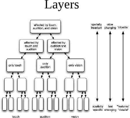
The Cortex Hawkins’s point of interest in the brain – “Where the magic happens” Hierarchically-arranged in regions Communication up the hierarchy – Regions classify patterns of their inputs – Regions output a ‘named’ pattern up the hierarchy Communication down the hierarchy – A high-level region has made a prediction – Alerts lower-level regions what to expect
Hawkins Quotes “The human cortex is particularly large and therefore has a massive memory capacity. It is constantly predicting what you will see, hear and feel, mostly in ways you are unconscious of. These predictions are our thoughts, and when combined with sensory inputs, they are our perceptions. I call this view of the brain the memory-prediction framework of intelligence.”
Hawkins Quotes “Your brain constantly makes predictions about the very fabric of the world we live in, and it does so in a parallel fashion. It will just as readily detect an odd texture, a misshapen nose, or an unusual motion. It isn’t obvious how pervasive these mostly unconscious predictions are, which is perhaps why we missed their importance.”
Hawkins Quotes “Your brain constantly makes predictions about the very fabric of the world we live in, and it does so in a parallel fashion. It will just as readily detect an odd texture, a misshapen nose, or an unusual motion. It isn’t obvious how pervasive these mostly unconscious predictions are, which is perhaps why we missed their importance.”
Hawkins Quotes “Suppose when you are out, I sneak over to your home and change something about your door. It could be almost anything. I could move the knob over by and inch, change a round knob into a thumb latch, or turn it from brass to chrome . When you come home that day and attempt to open the door, you will quickly detect that something is wrong.”
Prediction Prediction means that the neurons involved in sensing your door become active in advance of them actually receiving sensory input. – When the sensory input does arrive, it is compared with what is expected. – Two way communication; classification up the hierarchy, prediction down the hierarchy
Prediction Prediction is not limited to patterns of low-level sensory information like hearing and seeing Mountcastle’s principle : we have lots of different neurons, but they basically do the same thing (particularly in the neocortex) – What is true of low-level sensory areas must be true for all cortical areas. The human brain is more intelligent than that of other animals because it can make predictions about more abstract kinds of patterns and longer temporal pattern sequences.”
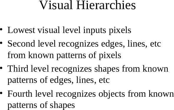
Visual Hierarchies Lowest visual level inputs pixels Second level recognizes edges, lines, etc from known patterns of pixels Third level recognizes shapes from known patterns of edges, lines, etc Fourth level recognizes objects from known patterns of shapes
Layers
Not there yet Many issues remain to be addressed by Hawkins’ model – Missing lots of details on how his model could be implemented in a computer – Creativity? – Evolution? – Planning? – Rest of the brain, not just neocortex?
Links and Examples http://davis.wpi.edu/ matt/courses/soms/ applet.html http://websom.hut.fi/websom/ milliondemo/html/root.html http://www.cis.hut.fi/research/somresearch/worldmap.html http://www.patol.com/java/TSP/index.html