Cost Behavior and Cost-Volume-Profit Analysis Chapter 18 Wild,


64 Slides6.02 MB
Cost Behavior and Cost-Volume-Profit Analysis Chapter 18 Wild, Shaw, and Chiappetta Financial and Managerial Accounting 7th Edition McGraw-Hill Education. All rights reserved. Authorized only for instructor use in the classroom. No reproduction or further distribution permitted without the prior written consent of McGraw-Hill Education.
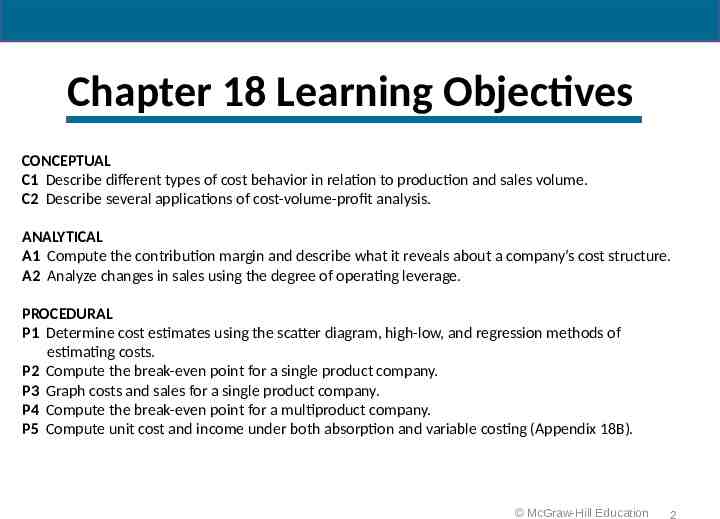
Chapter 18 Learning Objectives CONCEPTUAL C1 Describe different types of cost behavior in relation to production and sales volume. C2 Describe several applications of cost-volume-profit analysis. ANALYTICAL A1 Compute the contribution margin and describe what it reveals about a company’s cost structure. A2 Analyze changes in sales using the degree of operating leverage. PROCEDURAL P1 Determine cost estimates using the scatter diagram, high-low, and regression methods of estimating costs. P2 Compute the break-even point for a single product company. P3 Graph costs and sales for a single product company. P4 Compute the break-even point for a multiproduct company. P5 Compute unit cost and income under both absorption and variable costing (Appendix 18B). McGraw-Hill Education 2
Learning Objective C1: Describe different types of cost behavior in relation to production and sales volume. McGraw-Hill Education 3
Identifying Cost Behavior Managers use cost-volume-profit analysis to make predictions such as: – How many units must we sell to break-even? – How much does income increase if we install a new machine to reduce labor costs? – What is the change in income if selling prices decline and sales volume increases? – How will income change if we change the sales mix of our products or services? – What sales volume is needed to earn a target income? Learning Objective C1: Describe different types of cost behavior in relation to production and sales volume. McGraw-Hill Education 4
Fixed Costs Exhibit 18.2 McGraw-Hill Education Learning Objective C1: Describe different types of cost behavior in relation to production and sales volume. 5
Variable Costs Exhibit 18.2 McGraw-Hill Education Learning Objective C1: Describe different types of cost behavior in relation to production and sales volume. 6
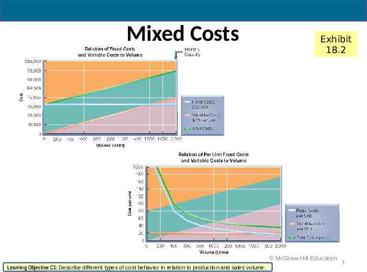
Mixed Costs Exhibit 18.2 McGraw-Hill Education Learning Objective C1: Describe different types of cost behavior in relation to production and sales volume. 7
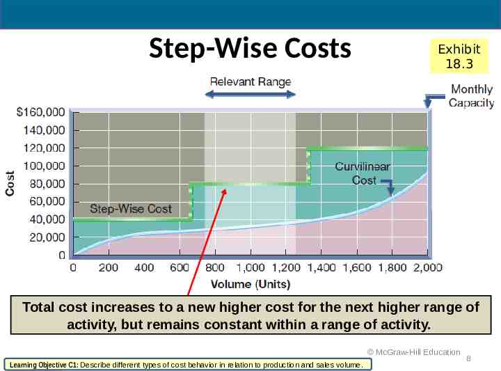
Step-Wise Costs Exhibit 18.3 Total cost increases to a new higher cost for the next higher range of activity, but remains constant within a range of activity. McGraw-Hill Education Learning Objective C1: Describe different types of cost behavior in relation to production and sales volume. 8
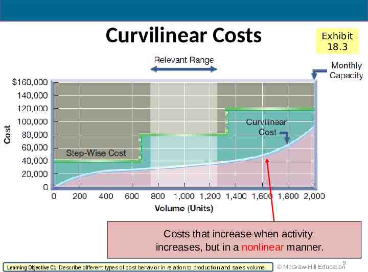
Curvilinear Costs Exhibit 18.3 Costs that increase when activity increases, but in a nonlinear manner. Learning Objective C1: Describe different types of cost behavior in relation to production and sales volume. 9 McGraw-Hill Education
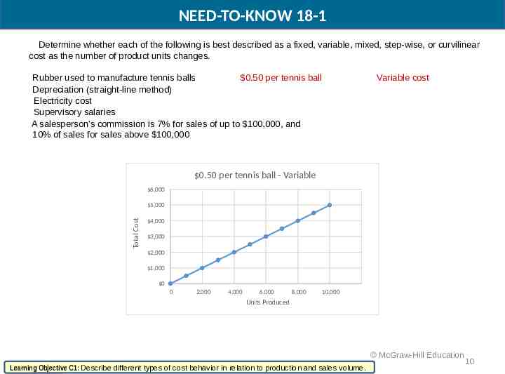
NEED-TO-KNOW 18-1 Determine whether each of the following is best described as a fixed, variable, mixed, step-wise, or curvilinear cost as the number of product units changes. Rubber used to manufacture tennis balls 0.50 per tennis ball Depreciation (straight-line method) Electricity cost Supervisory salaries A salesperson’s commission is 7% for sales of up to 100,000, and 10% of sales for sales above 100,000 Variable cost 0.50 per tennis ball - Variable 6,000 Total Cost 5,000 4,000 3,000 2,000 1,000 0 0 2,000 4,000 6,000 8,000 10,000 Units Produced McGraw-Hill Education Learning Objective C1: Describe different types of cost behavior in relation to production and sales volume. 10
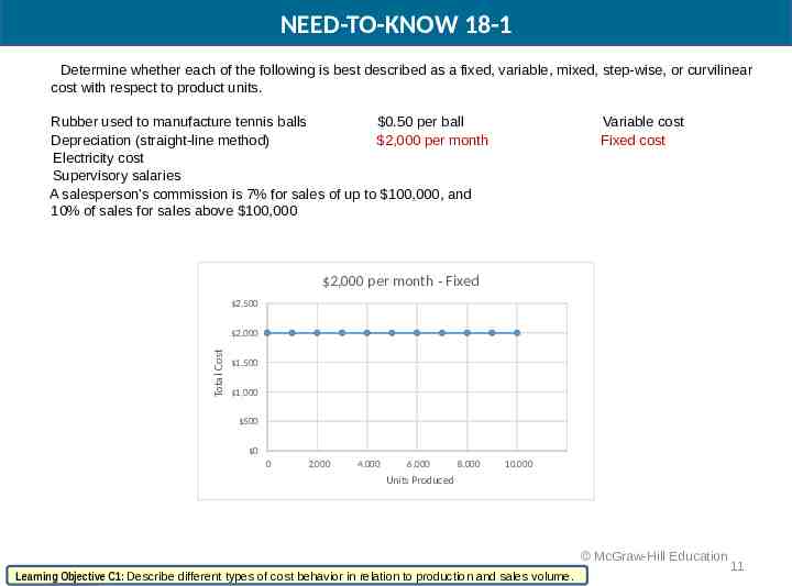
NEED-TO-KNOW 18-1 Determine whether each of the following is best described as a fixed, variable, mixed, step-wise, or curvilinear cost with respect to product units. Rubber used to manufacture tennis balls 0.50 per ball Depreciation (straight-line method) 2,000 per month Electricity cost Supervisory salaries A salesperson’s commission is 7% for sales of up to 100,000, and 10% of sales for sales above 100,000 Variable cost Fixed cost 2,000 per month - Fixed 2,500 Total Cost 2,000 1,500 1,000 500 0 0 2,000 4,000 6,000 8,000 10,000 Units Produced McGraw-Hill Education Learning Objective C1: Describe different types of cost behavior in relation to production and sales volume. 11
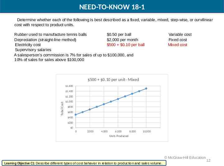
NEED-TO-KNOW 18-1 Determine whether each of the following is best described as a fixed, variable, mixed, step-wise, or curvilinear cost with respect to product units. Rubber used to manufacture tennis balls 0.50 per ball Depreciation (straight-line method) 2,000 per month Electricity cost 500 0.10 per ball Supervisory salaries A salesperson’s commission is 7% for sales of up to 100,000, and 10% of sales for sales above 100,000 Variable cost Fixed cost Mixed cost 500 0.10 per unit- Mixed 1,600 1,400 Total Cost 1,200 1,000 800 600 400 200 0 0 2,000 4,000 6,000 8,000 10,000 Units Produced McGraw-Hill Education Learning Objective C1: Describe different types of cost behavior in relation to production and sales volume. 12
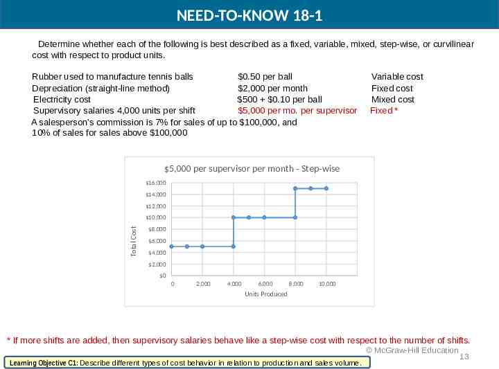
NEED-TO-KNOW 18-1 Determine whether each of the following is best described as a fixed, variable, mixed, step-wise, or curvilinear cost with respect to product units. Rubber used to manufacture tennis balls 0.50 per ball Depreciation (straight-line method) 2,000 per month Electricity cost 500 0.10 per ball Supervisory salaries 4,000 units per shift 5,000 per mo. per supervisor A salesperson’s commission is 7% for sales of up to 100,000, and 10% of sales for sales above 100,000 Variable cost Fixed cost Mixed cost Fixed * 5,000 per supervisor per month - Step-wise 16,000 14,000 12,000 Total Cost 10,000 8,000 6,000 4,000 2,000 0 0 2,000 4,000 6,000 8,000 10,000 Units Produced * If more shifts are added, then supervisory salaries behave like a step-wise cost with respect to the number of shifts. McGraw-Hill Education Learning Objective C1: Describe different types of cost behavior in relation to production and sales volume. 13
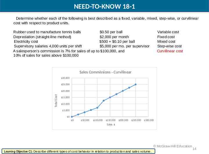
NEED-TO-KNOW 18-1 Determine whether each of the following is best described as a fixed, variable, mixed, step-wise, or curvilinear cost with respect to product units. Rubber used to manufacture tennis balls 0.50 per ball Depreciation (straight-line method) 2,000 per month Electricity cost 500 0.10 per ball Supervisory salaries 4,000 units per shift 5,000 per mo. per supervisor A salesperson’s commission is 7% for sales of up to 100,000, and 10% of sales for sales above 100,000 Variable cost Fixed cost Mixed cost Step-wise cost Curvilinear cost Sales Commissions - Curvilinear 30,000 25,000 Total Cost 20,000 15,000 10,000 5,000 0 0 50,000 100,000 150,000 200,000 250,000 300,000 Sales McGraw-Hill Education Learning Objective C1: Describe different types of cost behavior in relation to production and sales volume. 14
Learning Objective P1: Determine cost estimates using the scatter diagram, high-low, and regression methods of estimating costs. McGraw-Hill Education 15
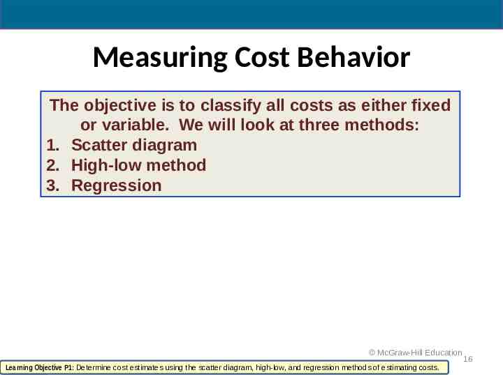
Measuring Cost Behavior The objective is to classify all costs as either fixed or variable. We will look at three methods: 1. Scatter diagram 2. High-low method 3. Regression McGraw-Hill Education Learning Objective P1: Determine cost estimates using the scatter diagram, high-low, and regression methods of estimating costs. 16
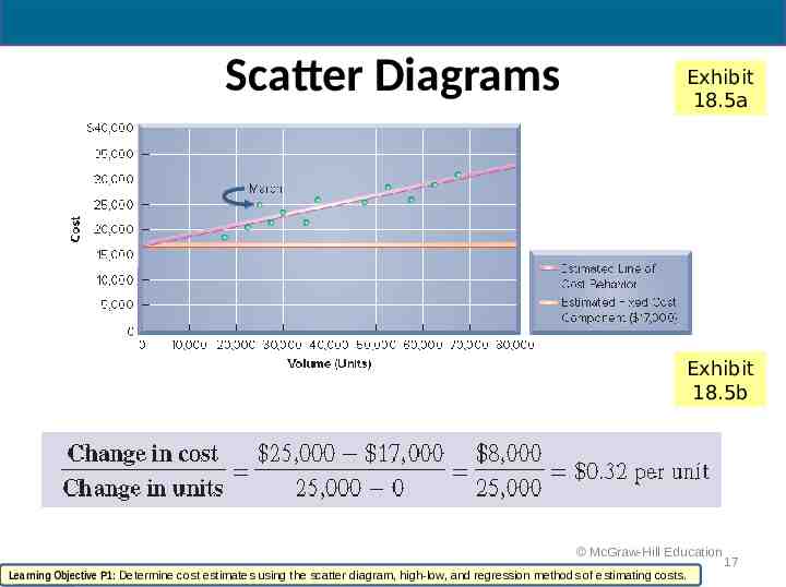
Scatter Diagrams Exhibit 18.5a Exhibit 18.5b McGraw-Hill Education Learning Objective P1: Determine cost estimates using the scatter diagram, high-low, and regression methods of estimating costs. 17
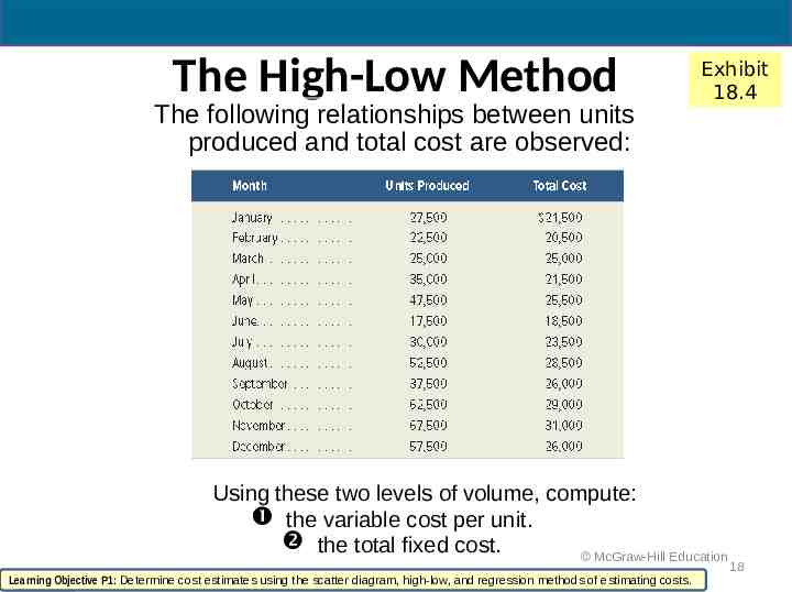
The High-Low Method The following relationships between units produced and total cost are observed: Exhibit 18.4 Using these two levels of volume, compute: the variable cost per unit. the total fixed cost. McGraw-Hill Education Learning Objective P1: Determine cost estimates using the scatter diagram, high-low, and regression methods of estimating costs. 18
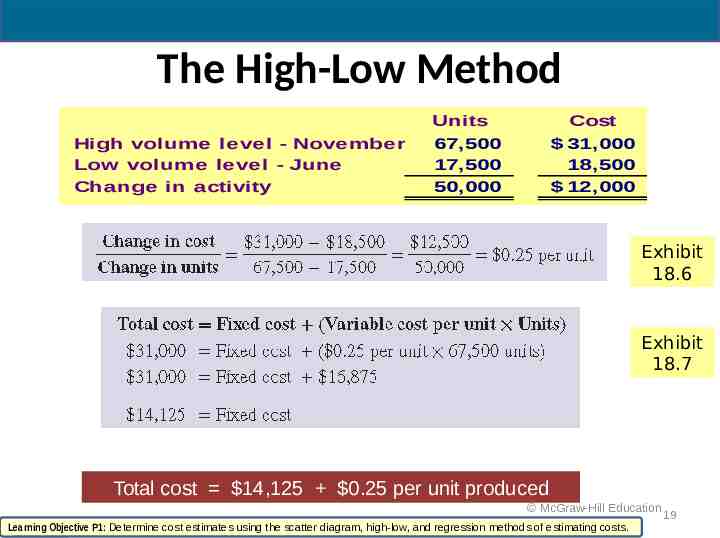
The High-Low Method High volume level - November Low volume level - June Change in activity Units 67,500 17,500 50,000 Cost 31,000 18,500 12,000 Exhibit 18.6 Exhibit 18.7 Total cost 14,125 0.25 per unit produced McGraw-Hill Education Learning Objective P1: Determine cost estimates using the scatter diagram, high-low, and regression methods of estimating costs. 19
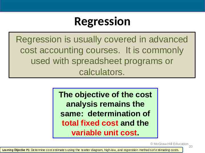
Regression Regression is usually covered in advanced cost accounting courses. It is commonly used with spreadsheet programs or calculators. The objective of the cost analysis remains the same: determination of total fixed cost and the variable unit cost. McGraw-Hill Education Learning Objective P1: Determine cost estimates using the scatter diagram, high-low, and regression methods of estimating costs. 20
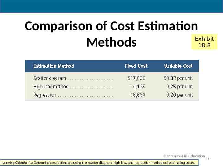
Comparison of Cost Estimation Exhibit Methods 18.8 McGraw-Hill Education Learning Objective P1: Determine cost estimates using the scatter diagram, high-low, and regression methods of estimating costs. 21
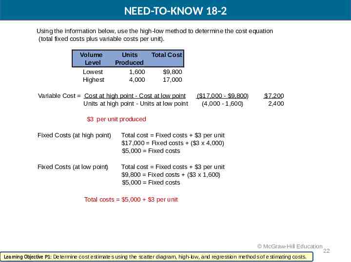
NEED-TO-KNOW 18-2 Using the information below, use the high-low method to determine the cost equation (total fixed costs plus variable costs per unit). Volume Level Lowest Highest Units Produced 1,600 4,000 Total Cost 9,800 17,000 Variable Cost Cost at high point - Cost at low point Units at high point - Units at low point ( 17,000 - 9,800) (4,000 - 1,600) 7,200 2,400 3 per unit produced Fixed Costs (at high point) Total cost Fixed costs 3 per unit 17,000 Fixed costs ( 3 x 4,000) 5,000 Fixed costs Fixed Costs (at low point) Total cost Fixed costs 3 per unit 9,800 Fixed costs ( 3 x 1,600) 5,000 Fixed costs Total costs 5,000 3 per unit McGraw-Hill Education Learning Objective P1: Determine cost estimates using the scatter diagram, high-low, and regression methods of estimating costs. 22
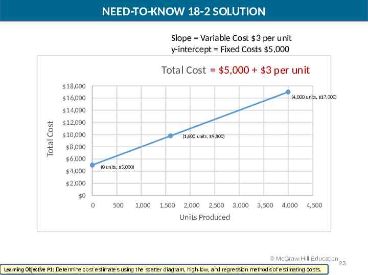
NEED-TO-KNOW 18-2 SOLUTION Slope Variable Cost 3 per unit y-intercept Fixed Costs 5,000 Total Cost 5,000 3 per unit 18,000 (4,000 units, 17,000) 16,000 Total Cost 14,000 12,000 10,000 (1,600 units, 9,800) 8,000 6,000 (0 units, 5,000) 4,000 2,000 0 0 500 1,000 1,500 2,000 2,500 3,000 3,500 4,000 4,500 Units Produced McGraw-Hill Education Learning Objective P1: Determine cost estimates using the scatter diagram, high-low, and regression methods of estimating costs. 23
Learning Objective A1: Compute the contribution margin and describe what it reveals about a company’s cost structure. McGraw-Hill Education 24
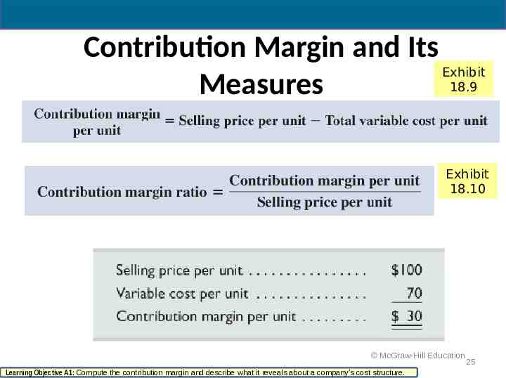
Contribution Margin and Its Exhibit 18.9 Measures Exhibit 18.10 McGraw-Hill Education Learning Objective A1: Compute the contribution margin and describe what it reveals about a company’s cost structure. 25
Learning Objective P2: Compute the break-even point for a single product company. McGraw-Hill Education 26
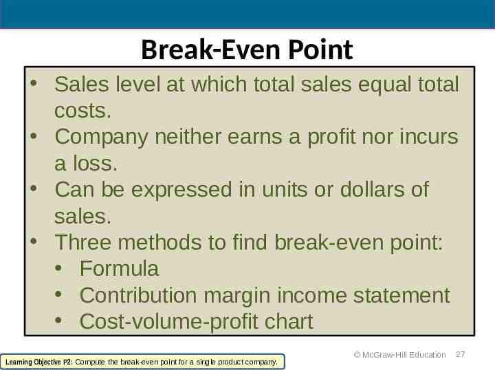
Break-Even Point Sales level at which total sales equal total costs. Company neither earns a profit nor incurs a loss. Can be expressed in units or dollars of sales. Three methods to find break-even point: Formula Contribution margin income statement Cost-volume-profit chart Learning Objective P2: Compute the break-even point for a single product company. McGraw-Hill Education 27
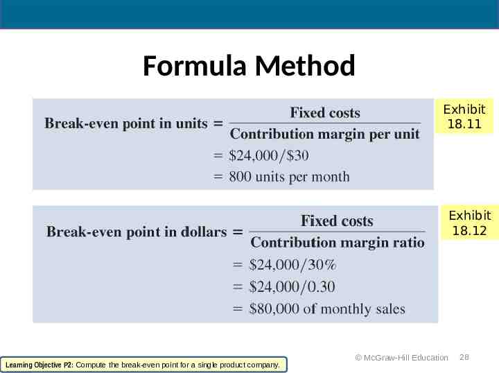
Formula Method Exhibit 18.11 Exhibit 18.12 Learning Objective P2: Compute the break-even point for a single product company. McGraw-Hill Education 28
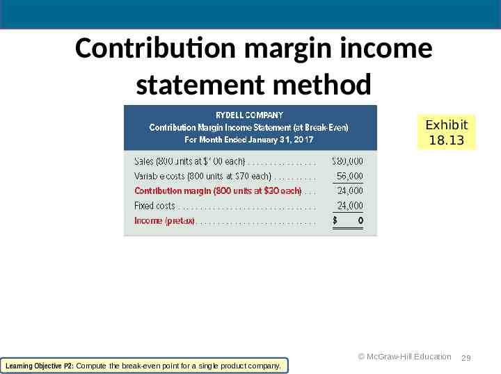
Contribution margin income statement method Exhibit 18.13 McGraw-Hill Education Learning Objective P2: Compute the break-even point for a single product company. 29
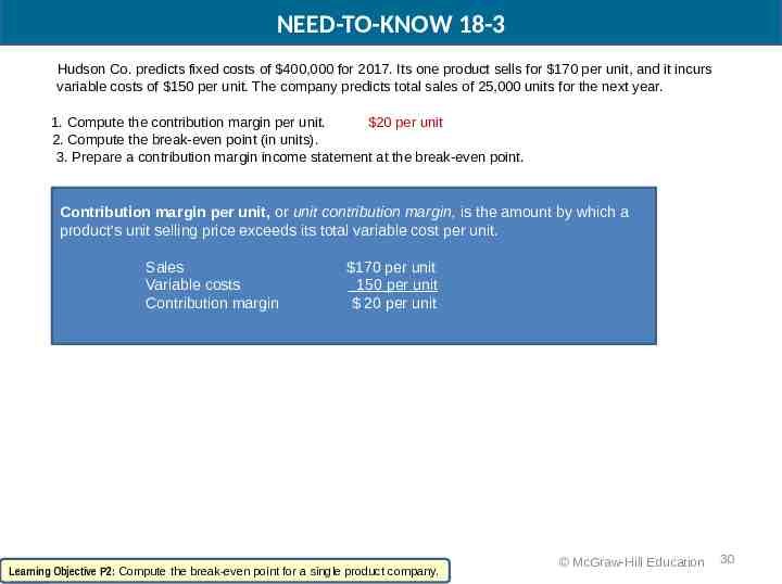
NEED-TO-KNOW 18-3 Hudson Co. predicts fixed costs of 400,000 for 2017. Its one product sells for 170 per unit, and it incurs variable costs of 150 per unit. The company predicts total sales of 25,000 units for the next year. 1. Compute the contribution margin per unit. 20 per unit 2. Compute the break-even point (in units). 3. Prepare a contribution margin income statement at the break-even point. Contribution margin per unit, or unit contribution margin, is the amount by which a product’s unit selling price exceeds its total variable cost per unit. Sales Variable costs Contribution margin 170 per unit 150 per unit 20 per unit Learning Objective P2: Compute the break-even point for a single product company. McGraw-Hill Education 30
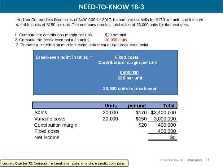
NEED-TO-KNOW 18-3 Hudson Co. predicts fixed costs of 400,000 for 2017. Its one product sells for 170 per unit, and it incurs variable costs of 150 per unit. The company predicts total sales of 25,000 units for the next year. 1. Compute the contribution margin per unit. 20 per unit 2. Compute the break-even point (in units). 20,000 units 3. Prepare a contribution margin income statement at the break-even point. Break-even point in units Fixed costs Contribution margin per unit 400,000 20 per unit 20,000 units to break-even Sales Variable costs Contribution margin Fixed costs Net income Units 20,000 20,000 Learning Objective P2: Compute the break-even point for a single product company. per unit Total 170 3,400,000 150 3,000,000 20 400,000 400,000 0 McGraw-Hill Education 31
Learning Objective P3: Graph costs and sales for a single product company. McGraw-Hill Education 32
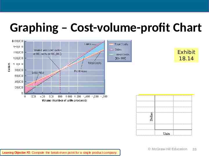
Graphing – Cost-volume-profit Chart Exhibit 18.14 Learning Objective P2: Compute the break-even point for a single product company. McGraw-Hill Education 33
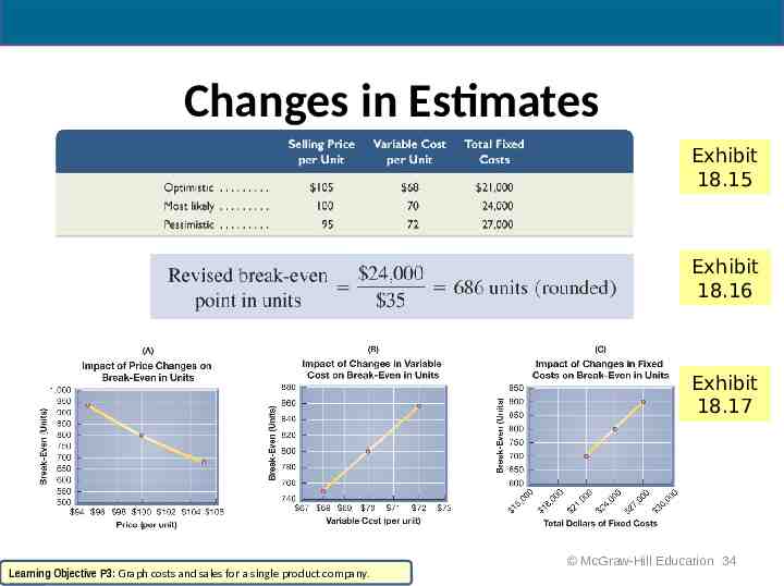
Changes in Estimates Exhibit 18.15 Exhibit 18.16 Exhibit 18.17 Learning Objective P3: Graph costs and sales for a single product company. McGraw-Hill Education 34
Learning Objective C2: Describe several applications of cost-volume-profit analysis. McGraw-Hill Education 35
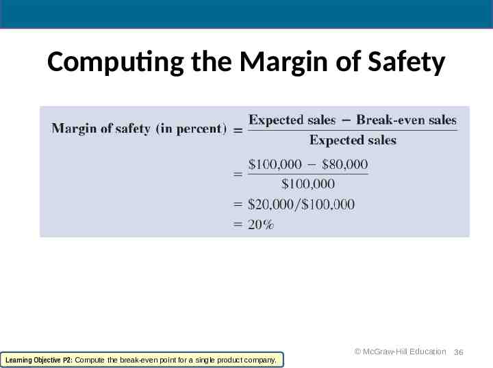
Computing the Margin of Safety Learning Objective P2: Compute the break-even point for a single product company. McGraw-Hill Education 36
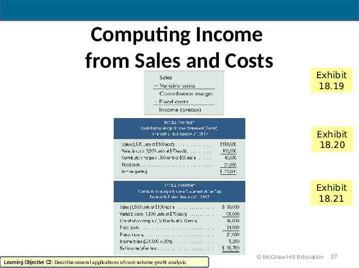
Computing Income from Sales and Costs Exhibit 18.19 Exhibit 18.20 Exhibit 18.21 Learning Objective C2: Describe several applications of cost-volume-profit analysis. McGraw-Hill Education 37
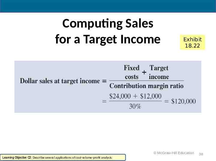
Computing Sales for a Target Income Exhibit 18.22 McGraw-Hill Education Learning Objective C2: Describe several applications of cost-volume-profit analysis. 38
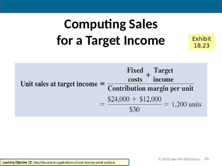
Computing Sales for a Target Income Learning Objective C2: Describe several applications of cost-volume-profit analysis. Exhibit 18.23 McGraw-Hill Education 39
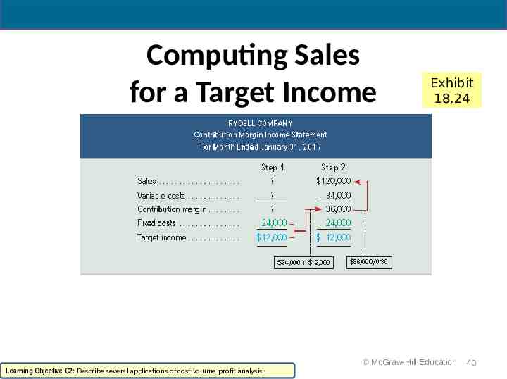
Computing Sales for a Target Income Learning Objective C2: Describe several applications of cost-volume-profit analysis. Exhibit 18.24 McGraw-Hill Education 40
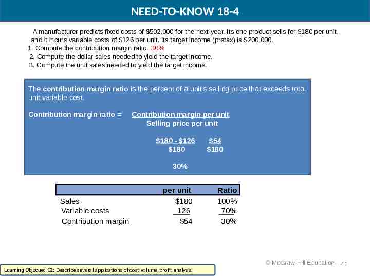
NEED-TO-KNOW 18-4 A manufacturer predicts fixed costs of 502,000 for the next year. Its one product sells for 180 per unit, and it incurs variable costs of 126 per unit. Its target income (pretax) is 200,000. 1. Compute the contribution margin ratio. 30% 2. Compute the dollar sales needed to yield the target income. 3. Compute the unit sales needed to yield the target income. The contribution margin ratio is the percent of a unit’s selling price that exceeds total unit variable cost. Contribution margin ratio Contribution margin per unit Selling price per unit 180 - 126 180 54 180 30% Sales Variable costs Contribution margin per unit 180 126 54 Ratio 100% 70% 30% McGraw-Hill Education Learning Objective C2: Describe several applications of cost-volume-profit analysis. 41
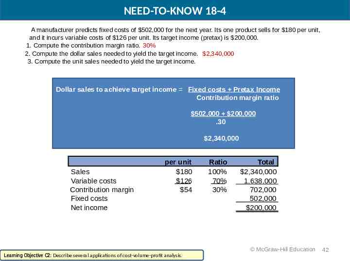
NEED-TO-KNOW 18-4 A manufacturer predicts fixed costs of 502,000 for the next year. Its one product sells for 180 per unit, and it incurs variable costs of 126 per unit. Its target income (pretax) is 200,000. 1. Compute the contribution margin ratio. 30% 2. Compute the dollar sales needed to yield the target income. 2,340,000 3. Compute the unit sales needed to yield the target income. Dollar sales to achieve target income Fixed costs Pretax Income Contribution margin ratio 502,000 200,000 .30 2,340,000 Sales Variable costs Contribution margin Fixed costs Net income per unit 180 126 54 Learning Objective C2: Describe several applications of cost-volume-profit analysis. Ratio 100% 70% 30% Total 2,340,000 1,638,000 702,000 502,000 200,000 McGraw-Hill Education 42
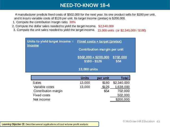
NEED-TO-KNOW 18-4 A manufacturer predicts fixed costs of 502,000 for the next year. Its one product sells for 180 per unit, and it incurs variable costs of 126 per unit. Its target income (pretax) is 200,000. 1. Compute the contribution margin ratio. 30% 2. Compute the dollar sales needed to yield the target income. 2,340,000 3. Compute the unit sales needed to yield the target income. 13,000 units (or 2,340,000 / 180) Units to yield target income Break-even point in units income Fixed costs target (pretax) Fixed costs Contribution margin per unit Contribution margin per unit 502,000 200,000 180 - 126 702,000 54 13,000 units Sales Variable costs Contribution margin Fixed costs Net income Units 13,000 13,000 Learning Objective C2: Describe several applications of cost-volume-profit analysis. per unit 180 126 54 Total 2,340,000 1,638,000 702,000 502,000 200,000 McGraw-Hill Education 43
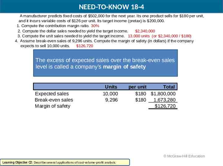
NEED-TO-KNOW 18-4 A manufacturer predicts fixed costs of 502,000 for the next year. Its one product sells for 180 per unit, and it incurs variable costs of 126 per unit. Its target income (pretax) is 200,000. 1. Compute the contribution margin ratio. 30% 2. Compute the dollar sales needed to yield the target income. 2,340,000 3. Compute the unit sales needed to yield the target income. 13,000 units (or 2,340,000 / 180) 4. Assume break-even sales of 9,296 units. Compute the margin of safety (in dollars) if the company expects to sell 10,000 units. 126,720 The excess of expected sales over the break-even sales level is called a company’s margin of safety Expected sales Break-even sales Margin of safety Units 10,000 9,296 per unit Total 180 1,800,000 180 1,673,280 126,720 McGraw-Hill Education Learning Objective C2: Describe several applications of cost-volume-profit analysis.
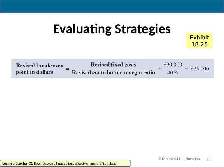
Evaluating Strategies Exhibit 18.25 McGraw-Hill Education Learning Objective C2: Describe several applications of cost-volume-profit analysis. 45
Learning Objective P4: Compute the break-even point for a multiproduct company. McGraw-Hill Education 46
Sales Mix and Break-Even The CVP formulas can be modified for use when a company sells more than one product. The unit contribution margin is replaced with the contribution margin for a composite unit. A composite unit is composed of specific numbers of each product in proportion to the product sales mix. Sales mix is the ratio of the volumes of the various products. Learning Objective P4: Compute the break-even point for a multiproduct company. McGraw-Hill Education 47
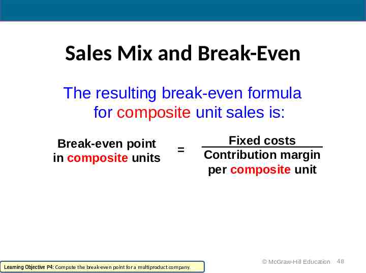
Sales Mix and Break-Even The resulting break-even formula for composite unit sales is: Break-even point in composite units Fixed costs Contribution margin per composite unit Continue Learning Objective P4: Compute the break-even point for a multiproduct company. McGraw-Hill Education 48
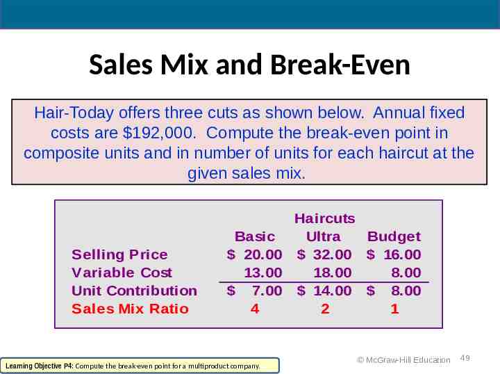
Sales Mix and Break-Even Hair-Today offers three cuts as shown below. Annual fixed costs are 192,000. Compute the break-even point in composite units and in number of units for each haircut at the given sales mix. Selling Price Variable Cost Unit Contribution Sales Mix Ratio Haircuts Basic Ultra Budget 20.00 32.00 16.00 13.00 18.00 8.00 7.00 14.00 8.00 4 2 1 Learning Objective P4: Compute the break-even point for a multiproduct company. McGraw-Hill Education 49
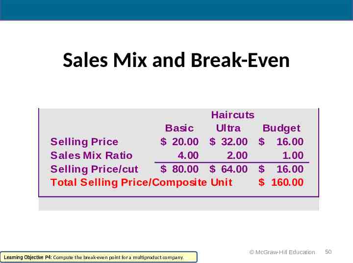
Sales Mix and Break-Even Haircuts Basic Ultra Selling Price 20.00 32.00 Sales Mix Ratio 4.00 2.00 Selling Price/cut 80.00 64.00 Total Selling Price/Composite Unit Learning Objective P4: Compute the break-even point for a multiproduct company. Budget 16.00 1.00 16.00 160.00 McGraw-Hill Education 50
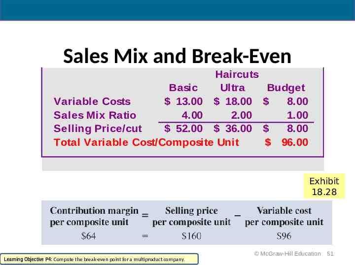
Sales Mix and Break-Even Haircuts Basic Ultra Variable Costs 13.00 18.00 Sales Mix Ratio 4.00 2.00 Selling Price/cut 52.00 36.00 Total Variable Cost/Composite Unit Budget 8.00 1.00 8.00 96.00 Exhibit 18.28 Learning Objective P4: Compute the break-even point for a multiproduct company. McGraw-Hill Education 51
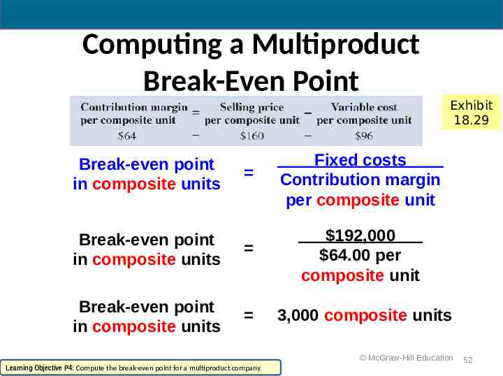
Computing a Multiproduct Break-Even Point Exhibit 18.29 Fixed costs Contribution margin per composite unit Break-even point in composite units 192,000 64.00 per composite unit Break-even point in composite units 3,000 composite units Break-even point in composite units McGraw-Hill Education Learning Objective P4: Compute the break-even point for a multiproduct company. 52
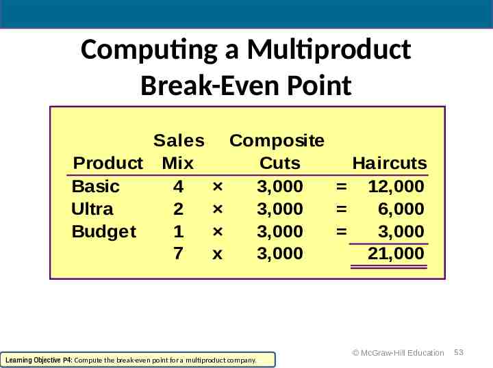
Computing a Multiproduct Break-Even Point Sales Product Mix Basic 4 Ultra 2 Budget 1 7 x Composite Cuts Haircuts 3,000 12,000 3,000 6,000 3,000 3,000 3,000 21,000 Learning Objective P4: Compute the break-even point for a multiproduct company. McGraw-Hill Education 53
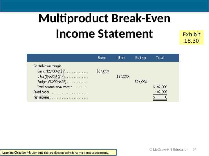
Multiproduct Break-Even Income Statement Learning Objective P4: Compute the break-even point for a multiproduct company. Exhibit 18.30 McGraw-Hill Education 54
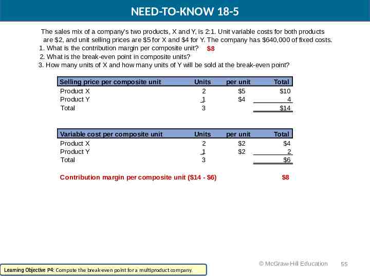
NEED-TO-KNOW 18-5 The sales mix of a company’s two products, X and Y, is 2:1. Unit variable costs for both products are 2, and unit selling prices are 5 for X and 4 for Y. The company has 640,000 of fixed costs. 1. What is the contribution margin per composite unit? 8 2. What is the break-even point in composite units? 3. How many units of X and how many units of Y will be sold at the break-even point? Selling price per composite unit Product X Product Y Total Units 2 1 3 per unit 5 4 Total 10 4 14 Variable cost per composite unit Product X Product Y Total Units 2 1 3 per unit 2 2 Total 4 2 6 Contribution margin per composite unit ( 14 - 6) Learning Objective P4: Compute the break-even point for a multiproduct company. 8 McGraw-Hill Education 55
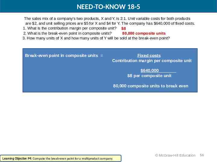
NEED-TO-KNOW 18-5 The sales mix of a company’s two products, X and Y, is 2:1. Unit variable costs for both products are 2, and unit selling prices are 5 for X and 4 for Y. The company has 640,000 of fixed costs. 1. What is the contribution margin per composite unit? 8 2. What is the break-even point in composite units? 80,000 composite units 3. How many units of X and how many units of Y will be sold at the break-even point? Break-even point in composite units Fixed costs Contribution margin per composite unit 640,000 8 per composite unit 80,000 composite units to break even Learning Objective P4: Compute the break-even point for a multiproduct company. McGraw-Hill Education 56
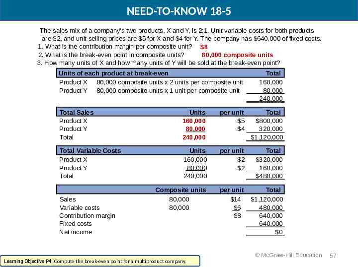
NEED-TO-KNOW 18-5 The sales mix of a company’s two products, X and Y, is 2:1. Unit variable costs for both products are 2, and unit selling prices are 5 for X and 4 for Y. The company has 640,000 of fixed costs. 1. What is the contribution margin per composite unit? 8 2. What is the break-even point in composite units? 80,000 composite units 3. How many units of X and how many units of Y will be sold at the break-even point? Units of each product at break-even Product X 80,000 composite units x 2 units per composite unit Product Y 80,000 composite units x 1 unit per composite unit Total 160,000 80,000 240,000 Total Sales Product X Product Y Total Units 160,000 80,000 240,000 per unit 5 4 Total 800,000 320,000 1,120,000 Total Variable Costs Product X Product Y Total Units 160,000 80,000 240,000 per unit 2 2 Total 320,000 160,000 480,000 Composite units 80,000 80,000 per unit 14 6 8 Total 1,120,000 480,000 640,000 640,000 0 Sales Variable costs Contribution margin Fixed costs Net income Learning Objective P4: Compute the break-even point for a multiproduct company. McGraw-Hill Education 57
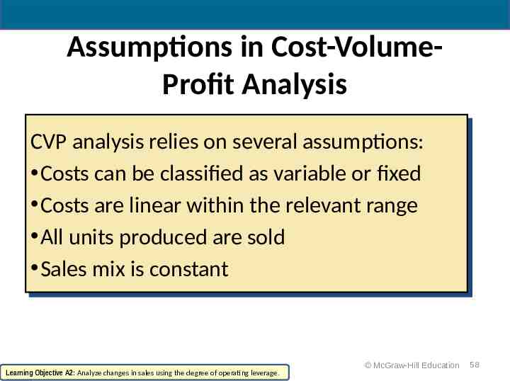
Assumptions in Cost-VolumeProfit Analysis CVP CVP analysis analysis relies relies on on several several assumptions: assumptions: Costs Costs can can be be classified classified as as variable variable or or fixed fixed Costs Costs are are linear linear within within the the relevant relevant range range All All units units produced produced are are sold sold Sales Sales mix mix isis constant constant Learning Objective A2: Analyze changes in sales using the degree of operating leverage. McGraw-Hill Education 58
Learning Objective A2: Analyze changes in sales using the degree of operating leverage. McGraw-Hill Education 59
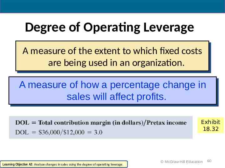
Degree of Operating Leverage AA measure measure of of the the extent extent to to which which fixed fixed costs costs are are being being used used in in an an organization. organization. AA measure measure of of how how aa percentage percentage change change in in sales sales will will affect affect profits. profits. Exhibit 18.32 Learning Objective A2: Analyze changes in sales using the degree of operating leverage. McGraw-Hill Education 60
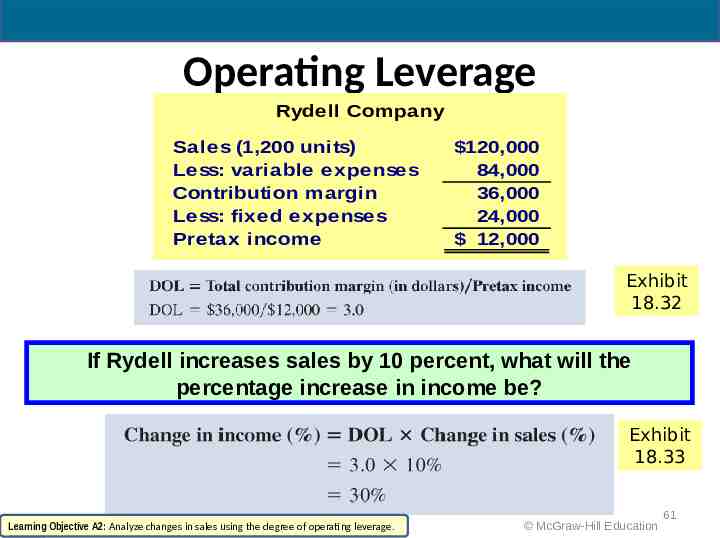
Operating Leverage Rydell Company Sales (1,200 units) Less: variable expenses Contribution margin Less: fixed expenses Pretax income 120,000 84,000 36,000 24,000 12,000 Exhibit 18.32 If Rydell increases sales by 10 percent, what will the percentage increase in income be? Exhibit 18.33 Learning Objective A2: Analyze changes in sales using the degree of operating leverage. McGraw-Hill Education 61
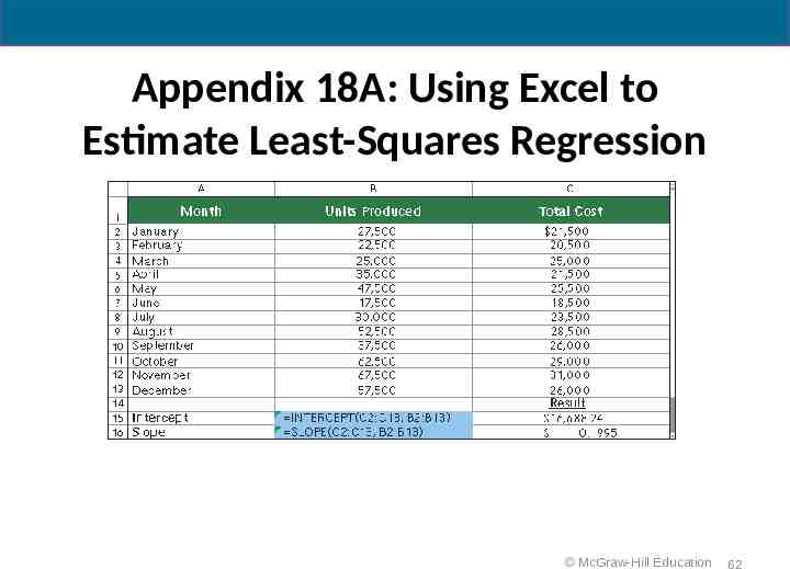
Appendix 18A: Using Excel to Estimate Least-Squares Regression McGraw-Hill Education 62
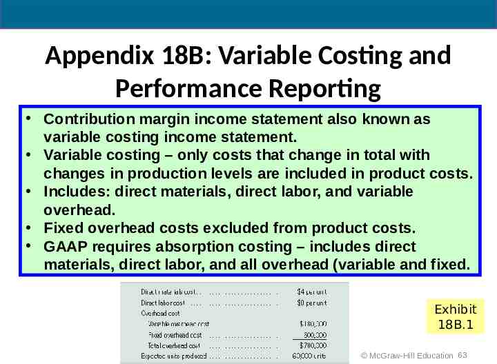
Appendix 18B: Variable Costing and Performance Reporting Contribution margin income statement also known as variable costing income statement. Variable costing – only costs that change in total with changes in production levels are included in product costs. Includes: direct materials, direct labor, and variable overhead. Fixed overhead costs excluded from product costs. GAAP requires absorption costing – includes direct materials, direct labor, and all overhead (variable and fixed. Exhibit 18B.1 McGraw-Hill Education 63
End of Chapter 18 McGraw-Hill Education 64