Portfolio Modeling with Time Dependent Correlation


42 Slides768.50 KB
Portfolio Modeling with Time Dependent Correlation Structure Computational Finance Rachel Chiu Sean Zeng Ricardo Affinito Sarah Thomas Dr. Katherine Ensor
Motivation “Risk management and oversight now focuses too much on the idiosyncratic risk that affects an individual firm and too little on the systematic issues that could affect market liquidity as a whole. To put it somewhat differently, the conventional risk-management framework today focuses too much on the threat to a firm from its own mistakes and too little on the potential for mistakes to be correlated across firms.” Timothy F. Geithner, President and CEO of the Federal Reserve Bank
Objective To develop a mixture model that captures the complex correlations present in a given portfolio
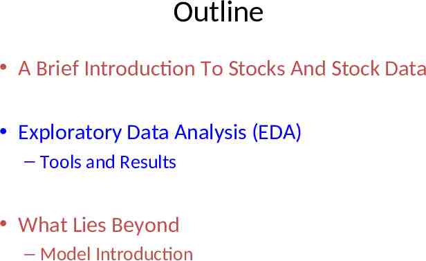
Outline A Brief Introduction To Stocks And Stock Data Exploratory Data Analysis (EDA) – Tools and Results What Lies Beyond – Model Introduction
Section 1 A BRIEF INTRODUCTION TO STOCKS AND STOCK DATA
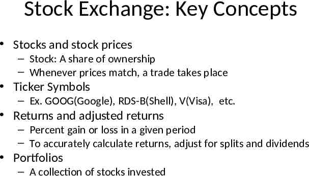
Stock Exchange: Key Concepts Stocks and stock prices – Stock: A share of ownership – Whenever prices match, a trade takes place Ticker Symbols – Ex. GOOG(Google), RDS-B(Shell), V(Visa), etc. Returns and adjusted returns – Percent gain or loss in a given period – To accurately calculate returns, adjust for splits and dividends Portfolios – A collection of stocks invested
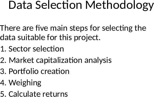
Data Selection Methodology There are five main steps for selecting the data suitable for this project. 1. Sector selection 2. Market capitalization analysis 3. Portfolio creation 4. Weighing 5. Calculate returns
Sector Selection Criteria History – Past performance and availability of data Sector characteristics – Startups vs. traditional Inter-relationship between the sectors – Ex. Oil Market Leaders and Solar - Positive – Ex. Oil Market Leaders and Airlines - Negative
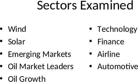
Sectors Examined Wind Solar Emerging Markets Oil Market Leaders Oil Growth Technology Finance Airline Automotive
Market Capitalization (MC) Seek companies that best represent the performance and characteristics of the chosen sector Formula: MC NSO SP – NSO Number of Shares Outstanding – SP Share Price Market capitalization the public opinion of a company’s net worth It helps us select the leaders in a sector
Portfolio Creation The stock market is too big; a portfolio limits the scope of the study A portfolio defines a pseudo world for complex correlations
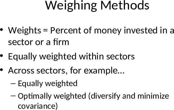
Weighing Methods Weights Percent of money invested in a sector or a firm Equally weighted within sectors Across sectors, for example – Equally weighted – Optimally weighted (diversify and minimize covariance)
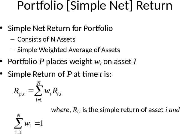
Portfolio [Simple Net] Return Simple Net Return for Portfolio – Consists of N Assets – Simple Weighted Average of Assets Portfolio P places weight wi on asset I Simple Return of P at time t is: N R p ,t wt Ri ,t i 1 where, Ri,t is the simple return of asset i and N w i i 1 1
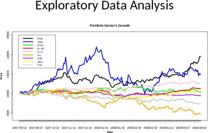
Exploratory Data Analysis 25000 Portfolio Sector's Growth Wind 20000 Solar Emkt Oil ML Oil G Airl Auto 15000 10000 5000 Price Tech Fina 2007-09-04 2007-09-27 2007-10-22 2007-11-14 2007-12-10 2008-01-04 2008-01-30 2008-02-25 2008-03-19 2008-04-14 2008-05-07 2008-06-02 Date
Outline A Brief Introduction To Stocks And Stock Data Exploratory Data Analysis (EDA) – Tools and Results What Lies Beyond – Model Introduction
Section 2 EXPLORATORY DATA ANALYSIS
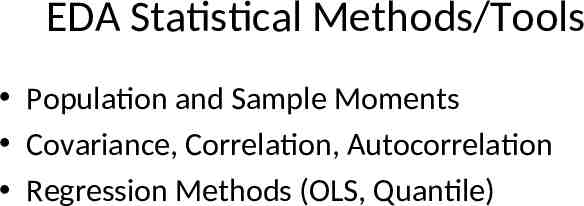
EDA Statistical Methods/Tools Population and Sample Moments Covariance, Correlation, Autocorrelation Regression Methods (OLS, Quantile)
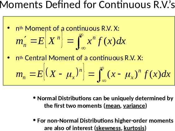
Moments Defined for Continuous R.V.’s nth Moment of a continuous R.V. X: x mn E X n n f ( x)dx nth Central Moment of a continuous R.V. X: n mn E X x ( x x ) n f ( x)dx Normal Distributions can be uniquely determined by the first two moments (mean, variance) For non-Normal Distributions higher-order moments are also of interest (skewness, kurtosis)
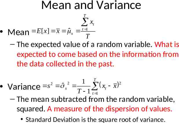
Mean and Variance T x Mean E[ x] x ˆ x t T1 t – The expected value of a random variable. What is expected to come based on the information from the data collected in the past. Variance s 2 ̂ x 2 1 T 2 x x t T 1 t 1 – The mean subtracted from the random variable, squared. A measure of the dispersion of values. Standard Deviation is the square root of variance.
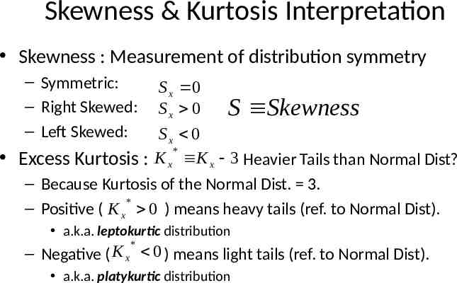
Skewness & Kurtosis Interpretation Skewness : Measurement of distribution symmetry – Symmetric: – Right Skewed: – Left Skewed: S x 0 Sx 0 S Skewness Sx 0 Excess Kurtosis : K x * K x 3 Heavier Tails than Normal Dist? – Because Kurtosis of the Normal Dist. 3. – Positive ( K x * 0 ) means heavy tails (ref. to Normal Dist). a.k.a. leptokurtic distribution * – Negative ( K x 0 ) means light tails (ref. to Normal Dist). a.k.a. platykurtic distribution
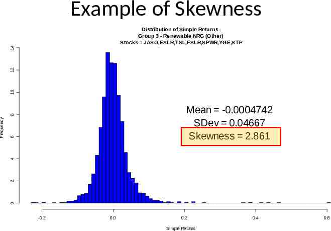
Example of Skewness 10 12 14 Distribution of Simple Returns Group 3 - Renewable NRG (Other) Stocks JASO,ESLR,TSL,FSLR,SPWR,YGE,STP Mean -0.0004742 SDev 0.04667 Skewness 2.861 6 4 2 0 Frequency 8 Mean -0.0004742 SDev 0.04667 Skewness 2.861 -0.2 0.0 0.2 Simple Returns 0.4 0.6
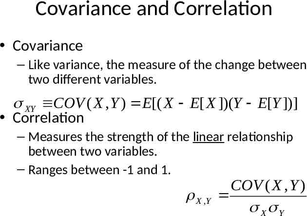
Covariance and Correlation Covariance – Like variance, the measure of the change between two different variables. XY COV ( X , Y ) E[( X E[ X ])(Y E[Y ])] Correlation – Measures the strength of the linear relationship between two variables. – Ranges between -1 and 1. X ,Y COV ( X , Y ) X Y
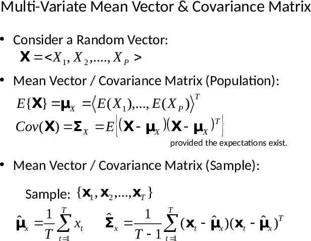
Multi-Variate Mean Vector & Covariance Matrix Consider a Random Vector: X X 1 , X 2 ,., X P Mean Vector / Covariance Matrix (Population): T E{X} μX E ( X 1 ),., E ( X P ) T Cov ( X) ΣX E X μX X μX provided the expectations exist. Mean Vector / Covariance Matrix (Sample): Sample: {x1 , x2 ,.,xT } T 1 T 1 T ˆ ˆ x xt ˆ ˆ μ Σ ( x μ ) ( x μ ) x t x t x T t 1 T 1 t 1
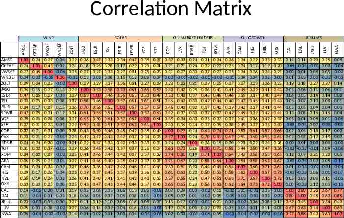
Correlation Matrix ZOLT JASO ESLR TSL FSLR SPWR YGE STP COP CVX RDS.B TOT XOM APA CAM HES NBL OXY CAL DAL JBLU LUV NWA AIRLINES WNDEF OIL GROWTH VWSYF OIL MARKET LEADERS GCTAF AMSC GCTAF VWSYF WNDEF ZOLT JASO ESLR TSL FSLR SPWR YGE STP COP CVX RDS.B TOT XOM APA CAM HES NBL OXY CAL DAL JBLU LUV NWA SOLAR AMSC WIND 1.00 0.24 0.27 0.04 0.29 0.36 0.47 0.33 0.34 0.47 0.39 0.37 0.37 0.33 0.24 0.31 0.34 0.36 0.34 0.29 0.35 0.33 0.14 0.11 0.20 0.25 0.05 0.24 1.00 0.45 0.02 0.24 0.18 0.25 0.28 0.17 0.29 0.28 0.31 0.21 0.21 0.24 0.32 0.22 0.25 0.24 0.17 0.19 0.20 -0.06 -0.04 -0.03 0.03 -0.04 0.27 0.45 1.00 -0.06 0.25 0.27 0.27 0.33 0.27 0.31 0.28 0.33 0.31 0.27 0.30 0.37 0.27 0.25 0.34 0.26 0.24 0.25 0.00 0.01 0.05 0.08 -0.02 0.04 0.02 -0.06 1.00 -0.02 0.13 0.03 0.08 0.15 0.12 0.08 0.07 0.00 -0.01 -0.02 -0.01 -0.02 -0.01 0.09 0.04 0.02 0.00 0.01 0.03 0.00 -0.02 -0.03 0.29 0.24 0.25 -0.02 1.00 0.29 0.29 0.37 0.36 0.31 0.27 0.29 0.28 0.23 0.21 0.29 0.25 0.27 0.27 0.23 0.26 0.25 0.19 0.18 0.27 0.27 0.14 0.36 0.18 0.27 0.13 0.29 1.00 0.53 0.58 0.70 0.61 0.65 0.59 0.43 0.42 0.29 0.36 0.41 0.41 0.46 0.39 0.41 0.43 0.05 0.06 0.11 0.06 0.01 0.47 0.25 0.27 0.03 0.29 0.53 1.00 0.46 0.56 0.55 0.50 0.48 0.50 0.42 0.37 0.45 0.46 0.46 0.36 0.37 0.40 0.47 0.06 0.05 0.19 0.14 0.02 0.33 0.28 0.33 0.08 0.37 0.58 0.46 1.00 0.52 0.51 0.61 0.51 0.46 0.43 0.33 0.42 0.44 0.40 0.47 0.45 0.41 0.43 0.05 0.07 0.10 0.09 0.01 0.34 0.17 0.27 0.15 0.36 0.70 0.56 0.52 1.00 0.57 0.57 0.57 0.45 0.42 0.32 0.37 0.42 0.39 0.42 0.37 0.41 0.44 0.05 0.05 0.09 0.04 0.03 0.47 0.29 0.31 0.12 0.31 0.61 0.55 0.51 0.57 1.00 0.57 0.63 0.42 0.37 0.33 0.37 0.37 0.42 0.46 0.39 0.42 0.44 0.13 0.08 0.16 0.16 0.04 0.39 0.28 0.28 0.08 0.27 0.65 0.50 0.61 0.57 0.57 1.00 0.61 0.39 0.34 0.33 0.35 0.37 0.37 0.41 0.36 0.42 0.37 0.05 0.01 0.09 0.01 -0.05 0.37 0.31 0.33 0.07 0.29 0.59 0.48 0.51 0.57 0.63 0.61 1.00 0.40 0.36 0.34 0.37 0.35 0.38 0.45 0.37 0.35 0.40 -0.08 -0.05 0.07 -0.08 -0.08 0.37 0.21 0.31 0.00 0.28 0.43 0.50 0.46 0.45 0.42 0.39 0.40 1.00 0.77 0.24 0.63 0.74 0.71 0.50 0.61 0.57 0.66 0.07 0.05 0.18 0.17 0.02 0.33 0.21 0.27 -0.01 0.23 0.42 0.42 0.43 0.42 0.37 0.34 0.36 0.77 1.00 0.24 0.70 0.81 0.67 0.51 0.60 0.55 0.65 0.09 0.07 0.17 0.19 0.03 0.24 0.24 0.30 -0.02 0.21 0.29 0.37 0.33 0.32 0.33 0.33 0.34 0.24 0.24 1.00 0.26 0.19 0.20 0.23 0.22 0.24 0.28 0.00 0.01 0.00 0.08 -0.03 0.31 0.32 0.37 -0.01 0.29 0.36 0.45 0.42 0.37 0.37 0.35 0.37 0.63 0.70 0.26 1.00 0.71 0.58 0.44 0.50 0.47 0.56 -0.02 -0.02 -0.01 0.09 -0.06 0.34 0.22 0.27 -0.02 0.25 0.41 0.46 0.44 0.42 0.37 0.37 0.35 0.74 0.81 0.19 0.71 1.00 0.64 0.48 0.58 0.53 0.63 0.12 0.09 0.21 0.22 0.05 0.36 0.25 0.25 -0.01 0.27 0.41 0.46 0.40 0.39 0.42 0.37 0.38 0.71 0.67 0.20 0.58 0.64 1.00 0.54 0.58 0.63 0.62 -0.02 -0.05 0.02 0.05 -0.13 0.34 0.24 0.34 0.09 0.27 0.46 0.36 0.47 0.42 0.46 0.41 0.45 0.50 0.51 0.23 0.44 0.48 0.54 1.00 0.60 0.71 0.64 0.01 -0.03 -0.02 -0.01 -0.04 0.29 0.17 0.26 0.04 0.23 0.39 0.37 0.45 0.37 0.39 0.36 0.37 0.61 0.60 0.22 0.50 0.58 0.58 0.60 1.00 0.67 0.73 -0.03 -0.03 0.06 0.01 -0.07 0.35 0.19 0.24 0.02 0.26 0.41 0.40 0.41 0.41 0.42 0.42 0.35 0.57 0.55 0.24 0.47 0.53 0.63 0.71 0.67 1.00 0.72 0.05 0.03 0.08 0.11 -0.03 0.33 0.20 0.25 0.00 0.25 0.43 0.47 0.43 0.44 0.44 0.37 0.40 0.66 0.65 0.28 0.56 0.63 0.62 0.64 0.73 0.72 1.00 0.00 -0.03 0.12 0.08 -0.10 0.14 -0.06 0.00 0.01 0.19 0.05 0.06 0.05 0.05 0.13 0.05 -0.08 0.07 0.09 0.00 -0.02 0.12 -0.02 0.01 -0.03 0.05 0.00 1.00 0.80 0.52 0.67 0.77 0.11 -0.04 0.01 0.03 0.18 0.06 0.05 0.07 0.05 0.08 0.01 -0.05 0.05 0.07 0.01 -0.02 0.09 -0.05 -0.03 -0.03 0.03 -0.03 0.80 1.00 0.45 0.63 0.86 0.20 -0.03 0.05 0.00 0.27 0.11 0.19 0.10 0.09 0.16 0.09 0.07 0.18 0.17 0.00 -0.01 0.21 0.02 -0.02 0.06 0.08 0.12 0.52 0.45 1.00 0.54 0.43 0.25 0.03 0.08 -0.02 0.27 0.06 0.14 0.09 0.04 0.16 0.01 -0.08 0.17 0.19 0.08 0.09 0.22 0.05 -0.01 0.01 0.11 0.08 0.67 0.63 0.54 1.00 0.60 0.05 -0.04 -0.02 -0.03 0.14 0.01 0.02 0.01 0.03 0.04 -0.05 -0.08 0.02 0.03 -0.03 -0.06 0.05 -0.13 -0.04 -0.07 -0.03 -0.10 0.77 0.86 0.43 0.60 1.00
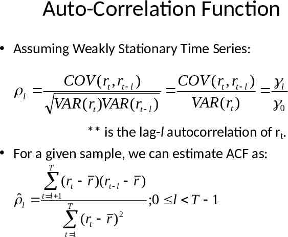
Auto-Correlation Function Assuming Weakly Stationary Time Series: COV ( rt , rt l ) COV ( rt , rt l ) l l VAR ( rt ) 0 VAR ( rt )VAR (rt l ) ** is the lag-l autocorrelation of rt. For a given sample, we can estimate ACF as: T (r r )(r t ˆ l t l 1 T t l 2 ( r r ) t t 1 r) ;0 l T 1
ACF Data Auto-Correlation Function (ACF) – The correlation of the data with itself, at different points in time. ACF lag1 lag2 lag3 lag4 WIND -0.02535 0.040051 -0.0392 0.017539 SOLAR 0.001937 -0.01604 -0.04285 -0.02221 EMKT -0.12514 -0.03283 0.115005 -0.12275 OILML OILG TECH FINA AIRL AUTO 0.098406 0.024246 -0.02548 0.149731 0.030379 -0.01032 0.028327 -0.0206 -0.02146 0.019471 -0.05436 0.039133 0.008292 -0.03115 -0.01141 -0.04077 0.001591 0.024963 -0.02576 -0.0132 -0.00852 -0.05975 -0.02699 0.043242
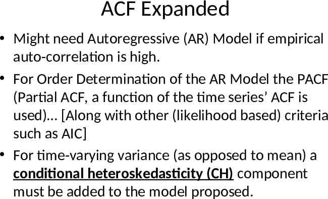
ACF Expanded Might need Autoregressive (AR) Model if empirical auto-correlation is high. For Order Determination of the AR Model the PACF (Partial ACF, a function of the time series’ ACF is used) [Along with other (likelihood based) criteria such as AIC] For time-varying variance (as opposed to mean) a conditional heteroskedasticity (CH) component must be added to the model proposed.
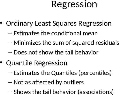
Regression Ordinary Least Squares Regression – Estimates the conditional mean – Minimizes the sum of squared residuals – Does not show the tail behavior Quantile Regression – Estimates the Quantiles (percentiles) – Not as affected by outliers – Shows the tail behavior (associations)
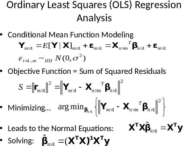
Ordinary Least Squares (OLS) Regression Analysis Conditional Mean Function Modeling T Ym 1 E[ Y X]m 1 εm 1 Xn m βn 1 εm 1 i 1.m IID N (0, 2 ) Objective Function Sum of Squared Residuals 2 T S rm 1 Ym 1 Xn m βn 1 2 2 T Minimizing arg min βn 1 Ym 1 Xn m βn 1 T T ˆ X Xβn 1 X y Leads to the Normal Equations: ˆ ( XT X)-1XT y Solving: β n 1
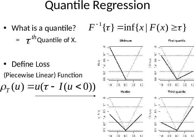
Quantile Regression What is a quantile? th F 1{ } inf{x F ( x) } Quantile of X. Define Loss for some (Piecewise Linear) Function T (u ) u ( I (u 0)) d d (0,1)
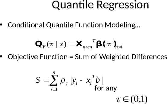
Quantile Regression Conditional Quantile Function Modeling T QY ( x ) Xn m β( )n 1 Objective Function Sum of Weighted Differences n T S yi xi b i 1 for any (0,1)
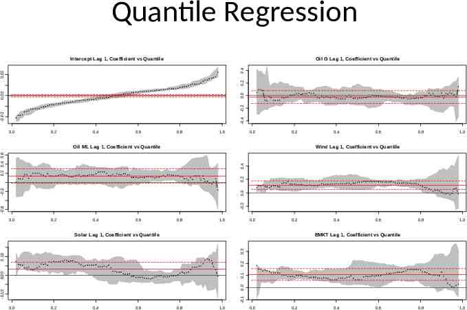
Quantile Regression Oil G Lag 1, Coefficient vs Quantile -0.4 -0.02 -0.2 0.0 0.00 0.2 0.02 0.4 Intercept Lag 1, Coefficient vs Quantile 0.0 0.2 0.4 0.6 0.8 1.0 0.0 0.2 0.6 0.8 1.0 0.8 1.0 0.8 1.0 Wind Lag 1, Coefficient vs Quantile -0.6 -0.2 0.0 -0.2 0.2 0.4 0.2 0.4 0.6 Oil ML Lag 1, Coefficient vs Quantile 0.4 0.0 0.2 0.4 0.6 0.8 1.0 0.0 0.2 0.6 EMKT Lag 1, Coefficient vs Quantile -0.1 -0.10 0.0 0.1 0.00 0.2 0.10 0.3 Solar Lag 1, Coefficient vs Quantile 0.4 0.0 0.2 0.4 0.6 0.8 1.0 0.0 0.2 0.4 0.6
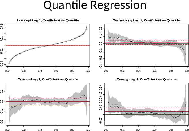
Quantile Regression Technology Lag 1, Coefficient vs Quantile -0.03 -0.01 -0.3 -0.2 -0.1 0.0 0.01 0.1 0.2 0.03 Intercept Lag 1, Coefficient vs Quantile 0.0 0.2 0.4 0.6 0.8 1.0 0.0 0.4 0.6 0.8 1.0 Energy Lag 1, Coefficient vs Quantile -0.2 -0.05 -0.1 0.0 0.1 0.05 0.10 0.15 0.20 Finance Lag 1, Coefficient vs Quantile 0.2 0.0 0.2 0.4 0.6 0.8 1.0 0.0 0.2 0.4 0.6 0.8 1.0
Quantile Regression Benefits Robust Estimation // Modeling Better View of Overall Portfolio Distribution as compared to conventional Conditional Mean Modeling. Explore Sources of Heterogeneity in the Portfolio Response (Observed Return)
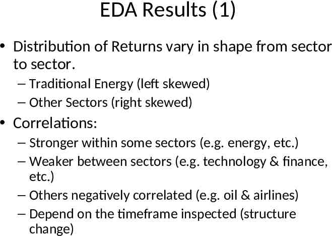
EDA Results (1) Distribution of Returns vary in shape from sector to sector. – Traditional Energy (left skewed) – Other Sectors (right skewed) Correlations: – Stronger within some sectors (e.g. energy, etc.) – Weaker between sectors (e.g. technology & finance, etc.) – Others negatively correlated (e.g. oil & airlines) – Depend on the timeframe inspected (structure change)
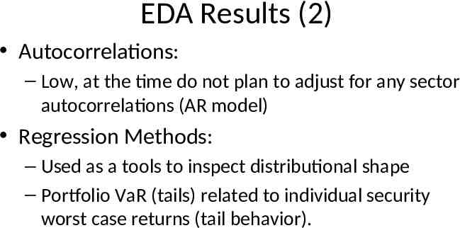
EDA Results (2) Autocorrelations: – Low, at the time do not plan to adjust for any sector autocorrelations (AR model) Regression Methods: – Used as a tools to inspect distributional shape – Portfolio VaR (tails) related to individual security worst case returns (tail behavior).
Outline A Brief Introduction To Stocks And Stock Data Exploratory Data Analysis (EDA) – Tools and Results What Lies Beyond – Model Introduction
Section 3 WHAT LIES BEYOND
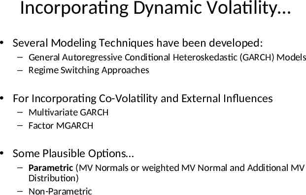
Incorporating Dynamic Volatility Several Modeling Techniques have been developed: – General Autoregressive Conditional Heteroskedastic (GARCH) Models – Regime Switching Approaches For Incorporating Co-Volatility and External Influences – Multivariate GARCH – Factor MGARCH Some Plausible Options – Parametric (MV Normals or weighted MV Normal and Additional MV Distribution) – Non-Parametric
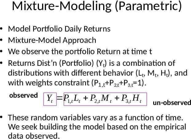
Mixture-Modeling (Parametric) Model Portfolio Daily Returns Mixture-Model Approach We observe the portfolio Return at time t Returns Dist’n (Portfolio) (Yt) is a combination of distributions with different behavior (Lt, Mt, Ht), and with weights constraint (P1,t P2,t P3,t 1). observed Yt P1,t Lt P2,t M t P3,t H t un-observed These random variables vary as a function of time. We seek building the model based on the empirical data observed.
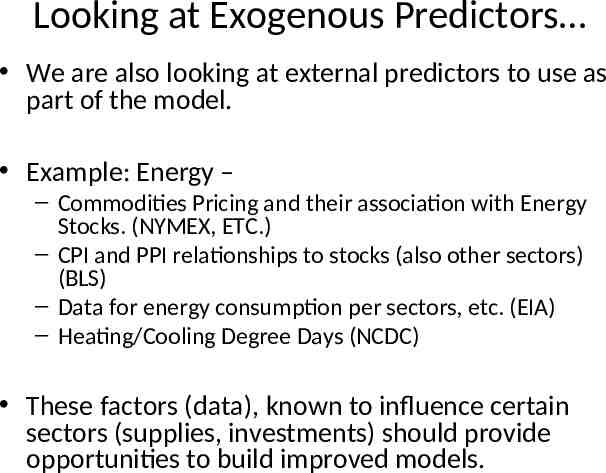
Looking at Exogenous Predictors We are also looking at external predictors to use as part of the model. Example: Energy – – Commodities Pricing and their association with Energy Stocks. (NYMEX, ETC.) – CPI and PPI relationships to stocks (also other sectors) (BLS) – Data for energy consumption per sectors, etc. (EIA) – Heating/Cooling Degree Days (NCDC) These factors (data), known to influence certain sectors (supplies, investments) should provide opportunities to build improved models.
Questions We would like to thank VIGRE, NSF, CoFES Please send any questions to Ricardo Affinito ([email protected]) Rachel Chiu ([email protected]) Sean Zeng ([email protected])