Distributed Computations MapReduce/Dryad M/R slides adapted from

Distributed Computations MapReduce/Dryad M/R slides adapted from those of Jeff Dean’s Dryad slides adapted from those of Michael Isard

What we’ve learnt so far Basic distributed systems concepts – Consistency (sequential, eventual) – Concurrency – Fault tolerance (recoverability, availability) What are distributed systems good for? – Better fault tolerance Better security? – Increased storage/serving capacity Storage systems, email clusters – Parallel (distributed) computation (Today’s topic)

Why distributed computations? How long to sort 1 TB on one computer? – One computer can read 60MB from disk – Takes 1 days!! Google indexes 100 billion web pages – 100 * 10 9 pages * 20KB/page 2 PB Large Hadron Collider is expected to produce 15 PB every year!

Solution: use many nodes! Cluster computing – Hundreds or thousands of PCs connected by high speed LANs Grid computing – Hundreds of supercomputers connected by high speed net 1000 nodes potentially give 1000X speedup

Distributed computations are difficult to program Sending data to/from nodes Coordinating among nodes Recovering from node failure Optimizing for locality Debugging Same for all problems

MapReduce A programming model for large-scale computations – Process large amounts of input, produce output – No side-effects or persistent state (unlike file system) MapReduce is implemented as a runtime library: – – – – automatic parallelization load balancing locality optimization handling of machine failures

MapReduce design Input data is partitioned into M splits Map: extract information on each split – Each Map produces R partitions Shuffle and sort – Bring M partitions to the same reducer Reduce: aggregate, summarize, filter or transform Output is in R result files

More specifically Programmer specifies two methods: – map(k, v) k', v' * – reduce(k', v' *) k', v' * All v' with same k' are reduced together, in order. Usually also specify: – partition(k’, total partitions) - partition for k’ often a simple hash of the key allows reduce operations for different k’ to be parallelized

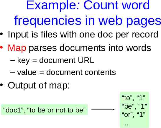
Example: Count word frequencies in web pages Input is files with one doc per record Map parses documents into words – key document URL – value document contents Output of map: “doc1”, “to be or not to be” “to”, “1” “be”, “1” “or”, “1”

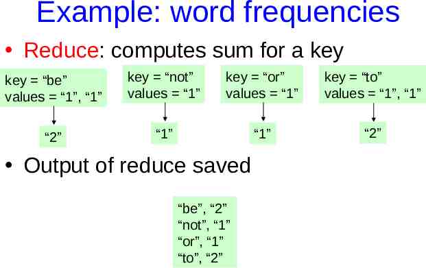
Example: word frequencies Reduce: computes sum for a key key “be” values “1”, “1” key “not” values “1” key “or” values “1” key “to” values “1”, “1” “2” “1” “1” “2” Output of reduce saved “be”, “2” “not”, “1” “or”, “1” “to”, “2”

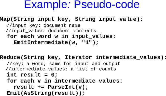
Example: Pseudo-code Map(String input key, String input value): //input key: document name //input value: document contents for each word w in input values: EmitIntermediate(w, "1"); Reduce(String key, Iterator intermediate values): //key: a word, same for input and output //intermediate values: a list of counts int result 0; for each v in intermediate values: result ParseInt(v); Emit(AsString(result));

MapReduce is widely applicable Distributed grep Document clustering Web link graph reversal Detecting approx. duplicate web pages

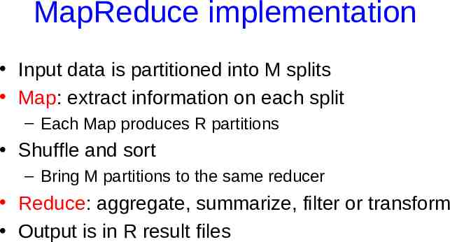
MapReduce implementation Input data is partitioned into M splits Map: extract information on each split – Each Map produces R partitions Shuffle and sort – Bring M partitions to the same reducer Reduce: aggregate, summarize, filter or transform Output is in R result files

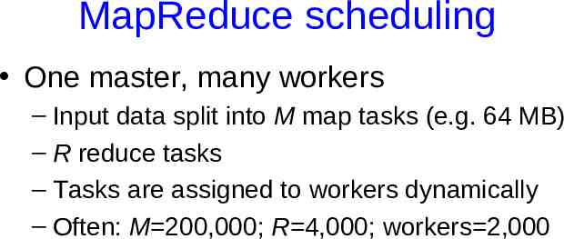
MapReduce scheduling One master, many workers – Input data split into M map tasks (e.g. 64 MB) – R reduce tasks – Tasks are assigned to workers dynamically – Often: M 200,000; R 4,000; workers 2,000

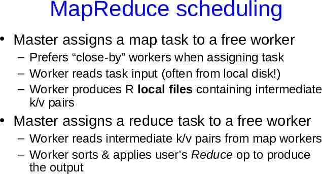
MapReduce scheduling Master assigns a map task to a free worker – Prefers “close-by” workers when assigning task – Worker reads task input (often from local disk!) – Worker produces R local files containing intermediate k/v pairs Master assigns a reduce task to a free worker – Worker reads intermediate k/v pairs from map workers – Worker sorts & applies user’s Reduce op to produce the output

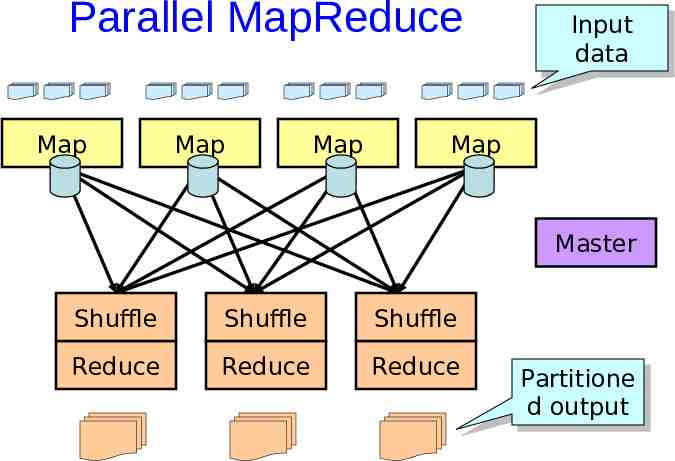
Parallel MapReduce Map Map Map Input Input data data Map Master Shuffle Shuffle Shuffle Reduce Reduce Reduce Partitione Partitione dd output output

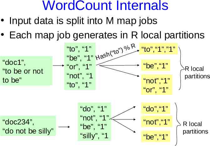
WordCount Internals Input data is split into M map jobs Each map job generates in R local partitions “doc1”, “to be or not to be” “doc234”, “do not be silly” R “to”,“1”,”1” % “to”, “1” ) ” (“to h s “be”, “1” Ha “be”,“1” “or”, “1” “not”, “1 “not”,“1” “to”, “1” “or”, “1” “do”, “1” “not”, “1” “be”, “1” “silly”, “1 R local partitions “do”,“1” “not”,“1” “be”,“1” R local partitions

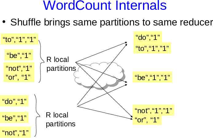
WordCount Internals Shuffle brings same partitions to same reducer “do”,“1” “to”,“1”,”1” “to”,“1”,”1” “be”,“1” “not”,“1” “or”, “1” R local partitions “be”,“1”,”1” “do”,“1” “be”,“1” “not”,“1” R local partitions “not”,“1”,”1” “or”, “1”

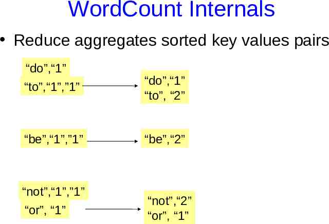
WordCount Internals Reduce aggregates sorted key values pairs “do”,“1” “to”,“1”,”1” “do”,“1” “to”, “2” “be”,“1”,”1” “be”,“2” “not”,“1”,”1” “or”, “1” “not”,“2” “or”, “1”

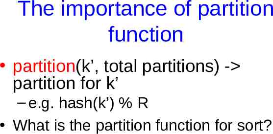
The importance of partition function partition(k’, total partitions) - partition for k’ – e.g. hash(k’) % R What is the partition function for sort?

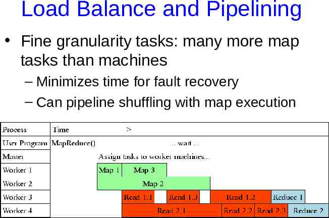
Load Balance and Pipelining Fine granularity tasks: many more map tasks than machines – Minimizes time for fault recovery – Can pipeline shuffling with map execution – Better dynamic load balancing Often use 200,000 map/5000 reduce tasks w/ 2000 machines

Fault tolerance via re-execution On worker failure: Re-execute completed and in-progress map tasks Re-execute in progress reduce tasks Task completion committed through master On master failure: State is checkpointed to GFS: new master recovers & continues

Avoid straggler using backup tasks Slow workers significantly lengthen completion time – – – – Other jobs consuming resources on machine Bad disks with soft errors transfer data very slowly Weird things: processor caches disabled (!!) An unusually large reduce partition? Solution: Near end of phase, spawn backup copies of tasks – Whichever one finishes first "wins" Effect: Dramatically shortens job completion time

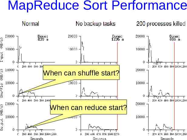
MapReduce Sort Performance 1TB (100-byte record) data to be sorted 1700 machines M 15000 R 4000

MapReduce Sort Performance When can shuffle start? When can reduce start?

Dryad Slides adapted from those of Yuan Yu and Michael Isard

Dryad Similar goals as MapReduce – focus on throughput, not latency – Automatic management of scheduling, distribution, fault tolerance Computations expressed as a graph – Vertices are computations – Edges are communication channels – Each vertex has several input and output edges

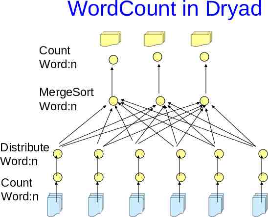
WordCount in Dryad Count Word:n MergeSort Word:n Distribute Word:n Count Word:n

Why using a dataflow graph? Many programs can be represented as a distributed dataflow graph – The programmer may not have to know this “SQL-like” queries: LINQ Dryad will run them for you

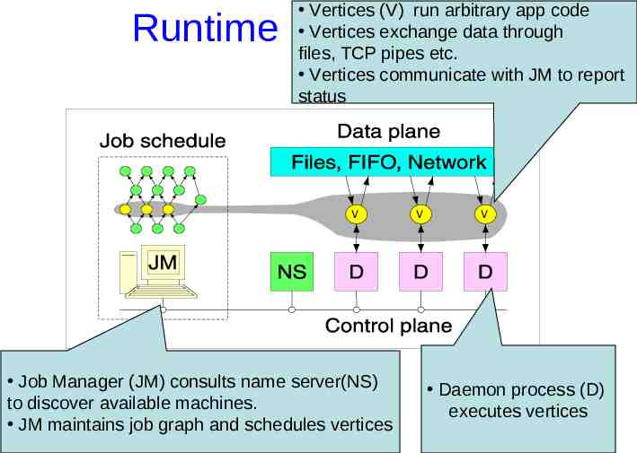
Runtime Vertices (V) run arbitrary app code Vertices exchange data through files, TCP pipes etc. Vertices communicate with JM to report status V Job Manager (JM) consults name server(NS) to discover available machines. JM maintains job graph and schedules vertices V V Daemon process (D) executes vertices

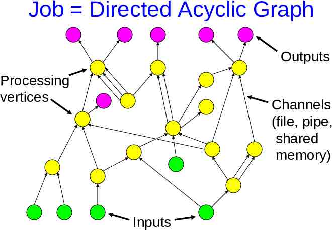
Job Directed Acyclic Graph Outputs Processing vertices Channels (file, pipe, shared memory) Inputs

Scheduling at JM General scheduling rules: – Vertex can run anywhere once all its inputs are ready Prefer executing a vertex near its inputs – Fault tolerance If A fails, run it again If A’s inputs are gone, run upstream vertices again (recursively) If A is slow, run another copy elsewhere and use output from whichever finishes first

Advantages of DAG over MapReduce Big jobs more efficient with Dryad – MapReduce: big job runs 1 MR stages reducers of each stage write to replicated storage Output of reduce: 2 network copies, 3 disks – Dryad: each job is represented with a DAG intermediate vertices write to local file

Advantages of DAG over MapReduce Dryad provides explicit join – MapReduce: mapper (or reducer) needs to read from shared table(s) as a substitute for join – Dryad: explicit join combines inputs of different types Dryad “Split” produces outputs of different types – Parse a document, output text and references

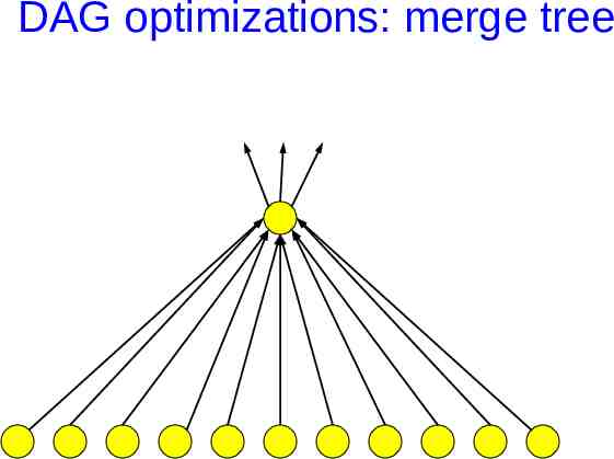
DAG optimizations: merge tree

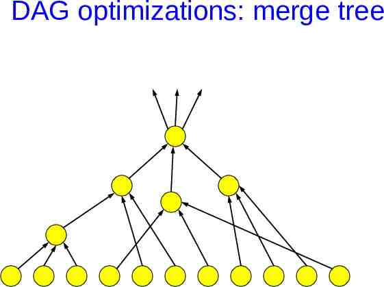
DAG optimizations: merge tree

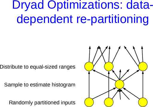
Dryad Optimizations: datadependent re-partitioning Distribute to equal-sized ranges Sample to estimate histogram Randomly partitioned inputs

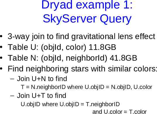
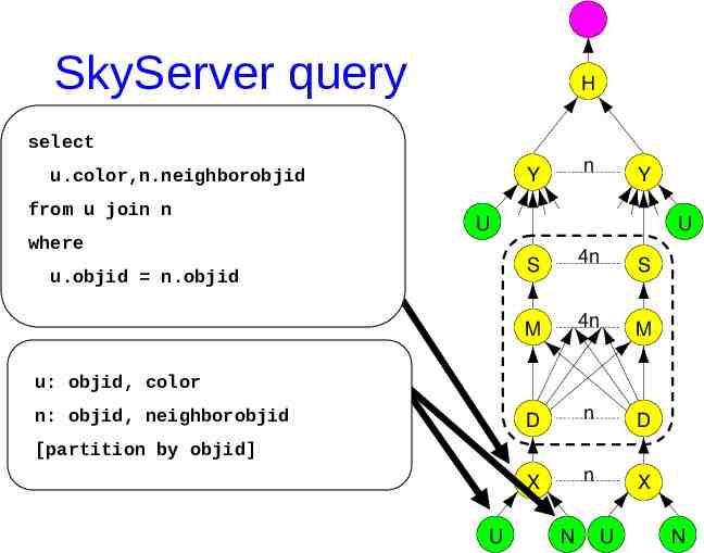
Dryad example 1: SkyServer Query 3-way join to find gravitational lens effect Table U: (objId, color) 11.8GB Table N: (objId, neighborId) 41.8GB Find neighboring stars with similar colors: – Join U N to find T N.neighborID where U.objID N.objID, U.color – Join U T to find U.objID where U.objID T.neighborID and U.color T.color

SkyServer query H select u.color,n.neighborobjid from u join n where n Y Y U u.objid n.objid U S 4n S M 4n M D n D X n X u: objid, color n: objid, neighborobjid [partition by objid] U N U N

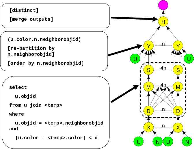
[distinct] [merge outputs] H (u.color,n.neighborobjid) [re-partition by n.neighborobjid] [order by n.neighborobjid] n Y Y U U S 4n S M 4n M where D n D u.objid temp .neighborobjid and X n X select u.objid from u join temp u.color - temp .color d U N U N

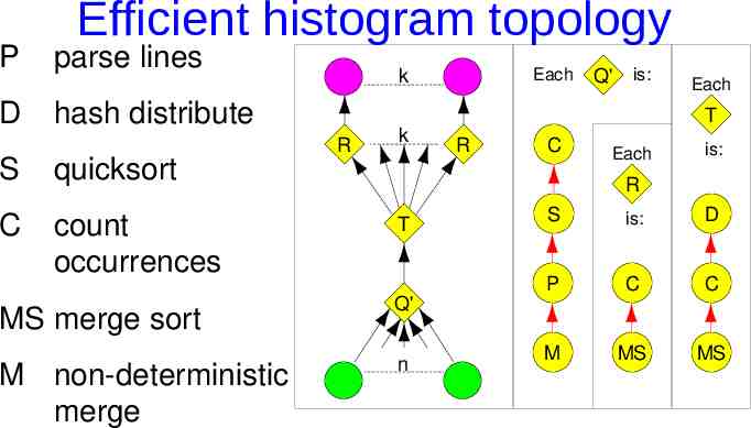
Dryad example 2: Query histogram computation Input: log file (n partitions) Extract queries from log partitions Re-partition by hash of query (k buckets) Compute histogram within each bucket

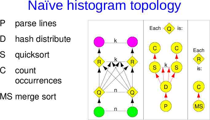
Naïve histogram topology P parse lines D hash distribute S Each C quicksort k R count occurrences MS merge sort is: k R C Q Q n n Q S C k Each R S is: D C P MS

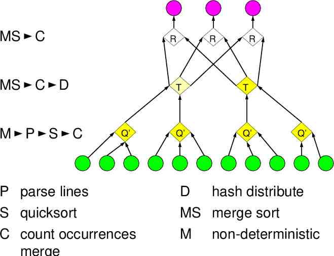
P D Efficient histogram topology parse lines hash distribute S quicksort C count occurrences MS merge sort M non-deterministic merge Each k R k Q' is: Each T R C Each is: R T Q' n S is: D P C C M MS MS

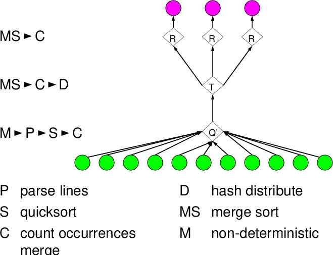
MS C R R MS C D T M P S C Q’ R P parse lines D hash distribute S quicksort MS merge sort C count occurrences merge M non-deterministic

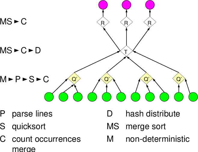
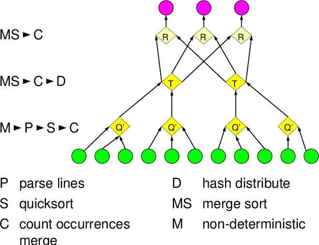
MS C R R MS C D M P S C R T Q’ Q’ Q’ P parse lines D S quicksort MS merge sort C count occurrences merge M Q’ hash distribute non-deterministic

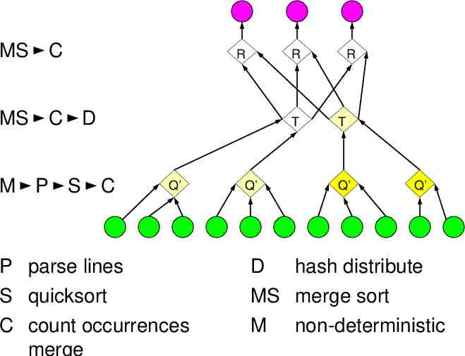
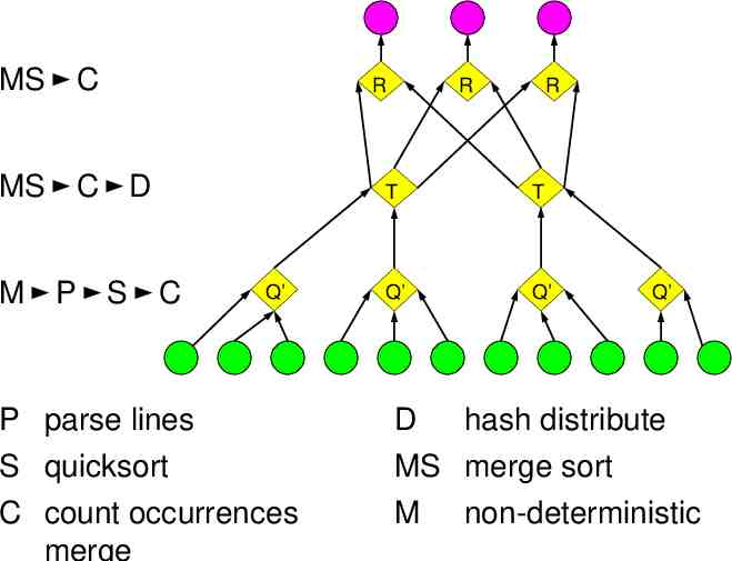
MS C R R MS C D M P S C T Q’ Q’ R T Q’ P parse lines D S quicksort MS merge sort C count occurrences merge M Q’ hash distribute non-deterministic

MS C R MS C D M P S C Q’ R R T T Q’ Q’ P parse lines D S quicksort MS merge sort C count occurrences merge M Q’ hash distribute non-deterministic

MS C R MS C D M P S C Q’ R R T T Q’ Q’ P parse lines D S quicksort MS merge sort C count occurrences merge M Q’ hash distribute non-deterministic

MS C R MS C D M P S C Q’ R R T T Q’ Q’ P parse lines D S quicksort MS merge sort C count occurrences merge M Q’ hash distribute non-deterministic

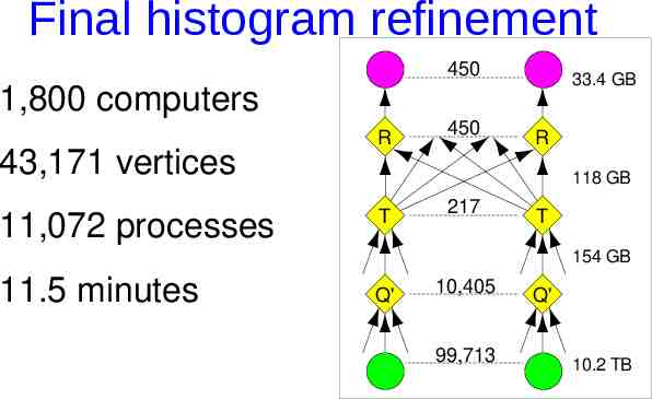
Final histogram refinement 450 33.4 GB 1,800 computers 43,171 vertices 11,072 processes R 450 R 118 GB T 217 T 154 GB 11.5 minutes Q' 10,405 99,713 Q' 10.2 TB