Data Mining: Concepts and Techniques (3rd ed.) — Chapter 4

58 Slides663.00 KB
Data Mining: Concepts and Techniques (3rd ed.) — Chapter 4 — Jiawei Han, Micheline Kamber, and Jian Pei University of Illinois at Urbana-Champaign & Simon Fraser University 2011 Han, Kamber & Pei. All rights reserved. 1
Chapter 4: Data Warehousing and On-line Analytical Processing Data Warehouse: Basic Concepts Data Warehouse Modeling: Data Cube and OLAP Data Warehouse Design and Usage Data Warehouse Implementation Data Generalization by Attribute-Oriented Induction Summary 2
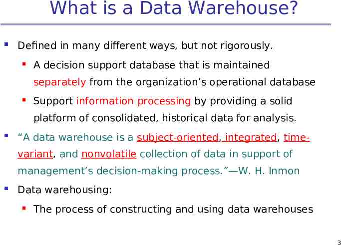
What is a Data Warehouse? Defined in many different ways, but not rigorously. A decision support database that is maintained separately from the organization’s operational database Support information processing by providing a solid platform of consolidated, historical data for analysis. “A data warehouse is a subject-oriented, integrated, timevariant, and nonvolatile collection of data in support of management’s decision-making process.”—W. H. Inmon Data warehousing: The process of constructing and using data warehouses 3
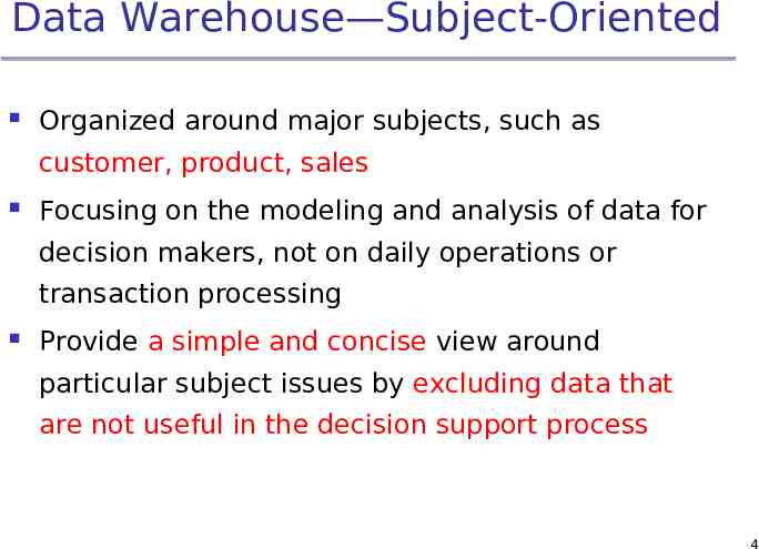
Data Warehouse—Subject-Oriented Organized around major subjects, such as customer, product, sales Focusing on the modeling and analysis of data for decision makers, not on daily operations or transaction processing Provide a simple and concise view around particular subject issues by excluding data that are not useful in the decision support process 4
Data Warehouse—Integrated Constructed by integrating multiple, heterogeneous data sources relational databases, flat files, on-line transaction records Data cleaning and data integration techniques are applied. Ensure consistency in naming conventions, encoding structures, attribute measures, etc. among different data sources E.g., Hotel price: currency, tax, breakfast covered, etc. When data is moved to the warehouse, it is converted. 5
Data Warehouse—Time Variant The time horizon for the data warehouse is significantly longer than that of operational systems Operational database: current value data Data warehouse data: provide information from a historical perspective (e.g., past 5-10 years) Every key structure in the data warehouse Contains an element of time, explicitly or implicitly But the key of operational data may or may not contain “time element” 6
Data Warehouse—Nonvolatile A physically separate store of data transformed from the operational environment Operational update of data does not occur in the data warehouse environment Does not require transaction processing, recovery, and concurrency control mechanisms Requires only two operations in data accessing: initial loading of data and access of data 7
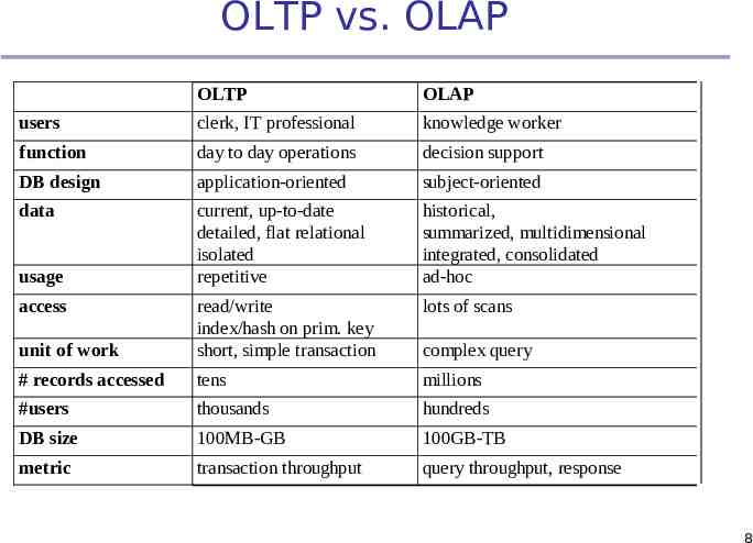
OLTP vs. OLAP OLTP OLAP users clerk, IT professional knowledge worker function day to day operations decision support DB design application-oriented subject-oriented data current, up-to-date detailed, flat relational isolated repetitive historical, summarized, multidimensional integrated, consolidated ad-hoc lots of scans unit of work read/write index/hash on prim. key short, simple transaction # records accessed tens millions #users thousands hundreds DB size 100MB-GB 100GB-TB metric transaction throughput query throughput, response usage access complex query 8
Why a Separate Data Warehouse? High performance for both systems Warehouse—tuned for OLAP: complex OLAP queries, multidimensional view, consolidation Different functions and different data: DBMS— tuned for OLTP: access methods, indexing, concurrency control, recovery missing data: Decision support requires historical data which operational DBs do not typically maintain data consolidation: DS requires consolidation (aggregation, summarization) of data from heterogeneous sources data quality: different sources typically use inconsistent data representations, codes and formats which have to be reconciled Note: There are more and more systems which perform OLAP analysis directly on relational databases 9
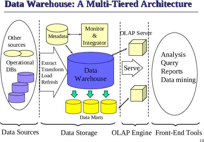
Data Warehouse: A Multi-Tiered Architecture Other sources Operational DBs Metadata Extract Transform Load Refresh Monitor & Integrator Data Warehouse OLAP Server Serve Analysis Query Reports Data mining Data Marts Data Sources Data Storage OLAP Engine Front-End Tools 10
Three Data Warehouse Models Enterprise warehouse collects all of the information about subjects spanning the entire organization Data Mart a subset of corporate-wide data that is of value to a specific groups of users. Its scope is confined to specific, selected groups, such as marketing data mart Independent vs. dependent (directly from warehouse) data mart Virtual warehouse A set of views over operational databases Only some of the possible summary views may be materialized 11
Extraction, Transformation, and Loading (ETL) Data extraction get data from multiple, heterogeneous, and external sources Data cleaning detect errors in the data and rectify them when possible Data transformation convert data from legacy or host format to warehouse format Load sort, summarize, consolidate, compute views, check integrity, and build indicies and partitions Refresh propagate the updates from the data sources to the warehouse 12
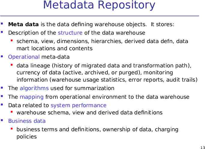
Metadata Repository Meta data is the data defining warehouse objects. It stores: Description of the structure of the data warehouse schema, view, dimensions, hierarchies, derived data defn, data mart locations and contents Operational meta-data data lineage (history of migrated data and transformation path), currency of data (active, archived, or purged), monitoring information (warehouse usage statistics, error reports, audit trails) The algorithms used for summarization The mapping from operational environment to the data warehouse Data related to system performance warehouse schema, view and derived data definitions Business data business terms and definitions, ownership of data, charging policies 13
Chapter 4: Data Warehousing and On-line Analytical Processing Data Warehouse: Basic Concepts Data Warehouse Modeling: Data Cube and OLAP Data Warehouse Design and Usage Data Warehouse Implementation Data Generalization by Attribute-Oriented Induction Summary 14
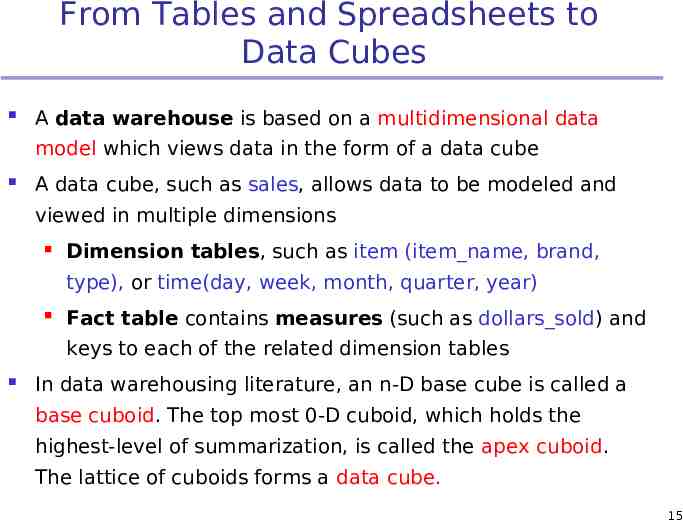
From Tables and Spreadsheets to Data Cubes A data warehouse is based on a multidimensional data model which views data in the form of a data cube A data cube, such as sales, allows data to be modeled and viewed in multiple dimensions Dimension tables, such as item (item name, brand, type), or time(day, week, month, quarter, year) Fact table contains measures (such as dollars sold) and keys to each of the related dimension tables In data warehousing literature, an n-D base cube is called a base cuboid. The top most 0-D cuboid, which holds the highest-level of summarization, is called the apex cuboid. The lattice of cuboids forms a data cube. 15
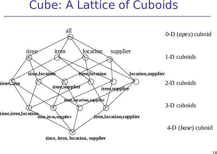
Cube: A Lattice of Cuboids all time 0-D (apex) cuboid item time,location time,item location supplier item,location time,supplier location,supplier item,supplier time,location,supplier time,item,location time,item,supplier 1-D cuboids 2-D cuboids 3-D cuboids item,location,supplier 4-D (base) cuboid time, item, location, supplier 16
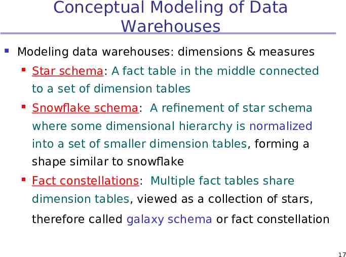
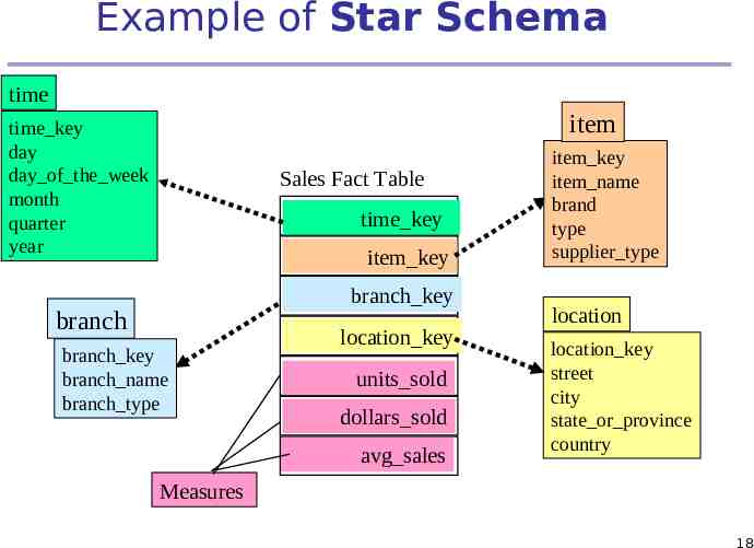
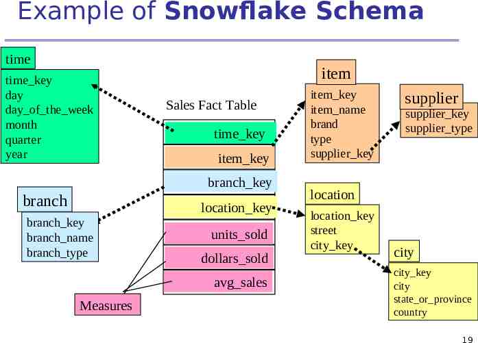
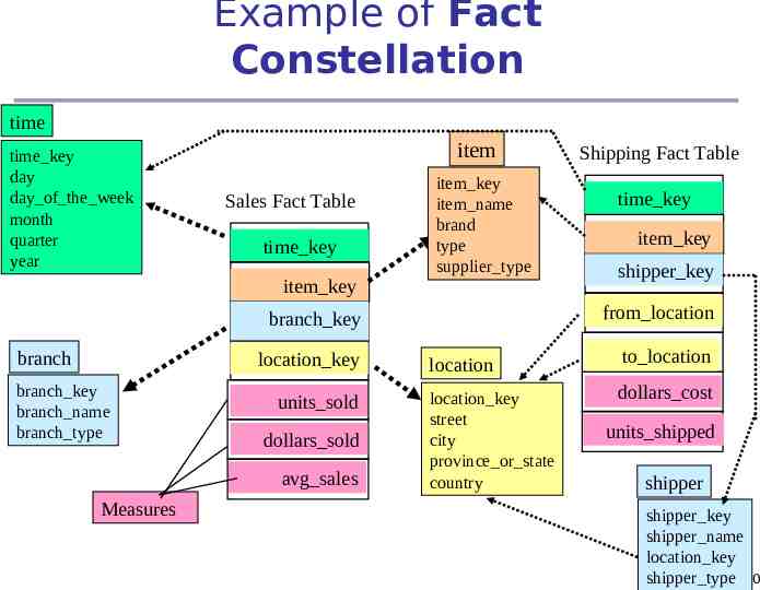
Conceptual Modeling of Data Warehouses Modeling data warehouses: dimensions & measures Star schema: A fact table in the middle connected to a set of dimension tables Snowflake schema: A refinement of star schema where some dimensional hierarchy is normalized into a set of smaller dimension tables, forming a shape similar to snowflake Fact constellations: Multiple fact tables share dimension tables, viewed as a collection of stars, therefore called galaxy schema or fact constellation 17
Example of Star Schema time item time key day day of the week month quarter year Sales Fact Table time key item key branch key branch branch key branch name branch type location key units sold dollars sold avg sales item key item name brand type supplier type location location key street city state or province country Measures 18
Example of Snowflake Schema time time key day day of the week month quarter year item Sales Fact Table time key item key branch key branch location key branch key branch name branch type units sold dollars sold avg sales Measures item key item name brand type supplier key supplier supplier key supplier type location location key street city key city city key city state or province country 19
Example of Fact Constellation time time key day day of the week month quarter year item Sales Fact Table time key item key item key item name brand type supplier type location key branch key branch name branch type units sold dollars sold avg sales Measures time key item key shipper key from location branch key branch Shipping Fact Table location to location location key street city province or state country dollars cost units shipped shipper shipper key shipper name location key shipper type 20
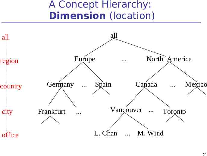
A Concept Hierarchy: Dimension (location) all all Europe region country city office Germany Frankfurt . . . Spain North America Canada Vancouver . L. Chan . Mexico Toronto . M. Wind 21
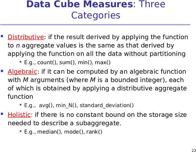
Data Cube Measures: Three Categories Distributive: if the result derived by applying the function to n aggregate values is the same as that derived by applying the function on all the data without partitioning Algebraic: if it can be computed by an algebraic function with M arguments (where M is a bounded integer), each of which is obtained by applying a distributive aggregate function E.g., count(), sum(), min(), max() E.g., avg(), min N(), standard deviation() Holistic: if there is no constant bound on the storage size needed to describe a subaggregate. E.g., median(), mode(), rank() 22
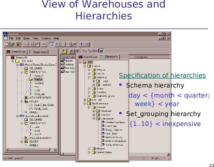
View of Warehouses and Hierarchies Specification of hierarchies Schema hierarchy day {month quarter; week} year Set grouping hierarchy {1.10} inexpensive 23
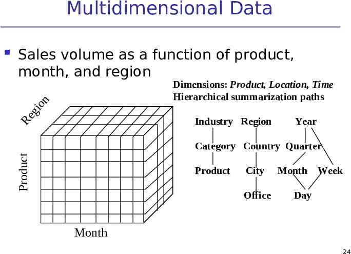
Multidimensional Data Sales volume as a function of product, month, and region Re gi on Dimensions: Product, Location, Time Hierarchical summarization paths Industry Region Year Category Country Quarter Product Product City Office Month Week Day Month 24
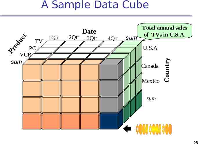
TV PC VCR sum 1Qtr 2Qtr Date 3Qtr 4Qtr sum Total annual sales of TVs in U.S.A. U.S.A Canada Mexico Country Pr od uc t A Sample Data Cube sum 25
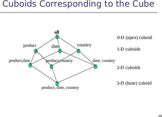
Cuboids Corresponding to the Cube all 0-D (apex) cuboid product product,date date country product,country 1-D cuboids date, country 2-D cuboids product, date, country 3-D (base) cuboid 26
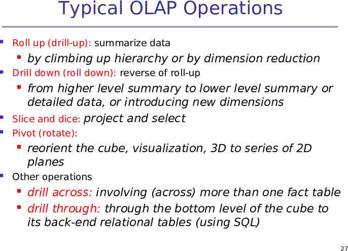
Typical OLAP Operations Roll up (drill-up): summarize data by climbing up hierarchy or by dimension reduction Drill down (roll down): reverse of roll-up from higher level summary to lower level summary or detailed data, or introducing new dimensions Slice and dice: project and select Pivot (rotate): reorient the cube, visualization, 3D to series of 2D planes Other operations drill across: involving (across) more than one fact table drill through: through the bottom level of the cube to its back-end relational tables (using SQL) 27
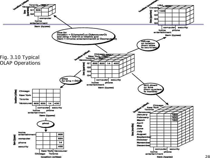
Fig. 3.10 Typical OLAP Operations 28
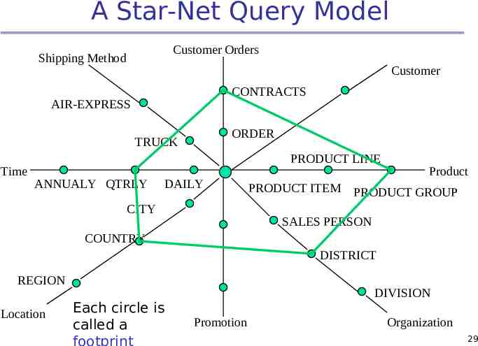
A Star-Net Query Model Customer Orders Shipping Method Customer CONTRACTS AIR-EXPRESS ORDER TRUCK Time PRODUCT LINE ANNUALY QTRLY DAILY CITY Product PRODUCT ITEM PRODUCT GROUP SALES PERSON COUNTRY DISTRICT REGION Location Each circle is called a footprint DIVISION Promotion Organization 29
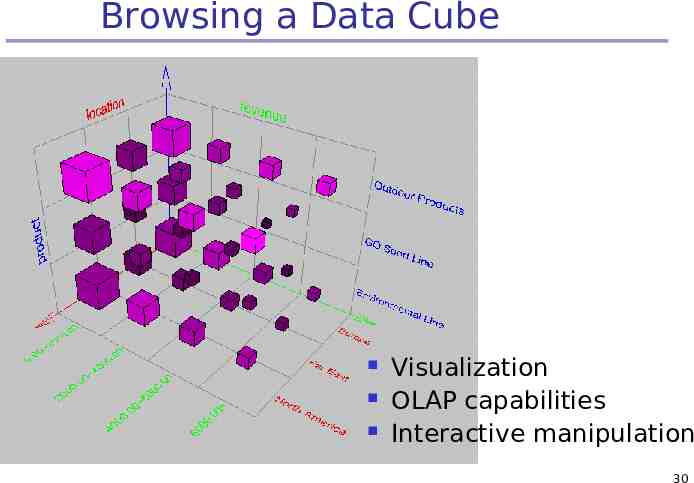
Browsing a Data Cube Visualization OLAP capabilities Interactive manipulation 30
Chapter 4: Data Warehousing and On-line Analytical Processing Data Warehouse: Basic Concepts Data Warehouse Modeling: Data Cube and OLAP Data Warehouse Design and Usage Data Warehouse Implementation Data Generalization by Attribute-Oriented Induction Summary 31
Design of Data Warehouse: A Business Analysis Framework Four views regarding the design of a data warehouse Top-down view Data source view exposes the information being captured, stored, and managed by operational systems Data warehouse view allows selection of the relevant information necessary for the data warehouse consists of fact tables and dimension tables Business query view sees the perspectives of data in the warehouse from the view of end-user 32
Data Warehouse Design Process Top-down, bottom-up approaches or a combination of both Top-down: Starts with overall design and planning (mature) Bottom-up: Starts with experiments and prototypes (rapid) From software engineering point of view Waterfall: structured and systematic analysis at each step before proceeding to the next Spiral: rapid generation of increasingly functional systems, short turn around time, quick turn around Typical data warehouse design process Choose a business process to model, e.g., orders, invoices, etc. Choose the grain (atomic level of data) of the business process Choose the dimensions that will apply to each fact table record Choose the measure that will populate each fact table record 33
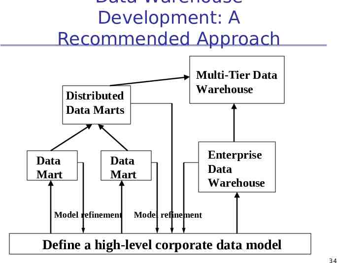
Data Warehouse Development: A Recommended Approach Multi-Tier Data Warehouse Distributed Data Marts Data Mart Data Mart Model refinement Enterprise Data Warehouse Model refinement Define a high-level corporate data model 34
Data Warehouse Usage Three kinds of data warehouse applications Information processing Analytical processing supports querying, basic statistical analysis, and reporting using crosstabs, tables, charts and graphs multidimensional analysis of data warehouse data supports basic OLAP operations, slice-dice, drilling, pivoting Data mining knowledge discovery from hidden patterns supports associations, constructing analytical models, performing classification and prediction, and presenting the mining results using visualization tools 35
From On-Line Analytical Processing (OLAP) to On Line Analytical Mining (OLAM) Why online analytical mining? High quality of data in data warehouses DW contains integrated, consistent, cleaned data Available information processing structure surrounding data warehouses ODBC, OLEDB, Web accessing, service facilities, reporting and OLAP tools OLAP-based exploratory data analysis Mining with drilling, dicing, pivoting, etc. On-line selection of data mining functions Integration and swapping of multiple mining functions, algorithms, and tasks 36
Chapter 4: Data Warehousing and On-line Analytical Processing Data Warehouse: Basic Concepts Data Warehouse Modeling: Data Cube and OLAP Data Warehouse Design and Usage Data Warehouse Implementation Data Generalization by Attribute-Oriented Induction Summary 37
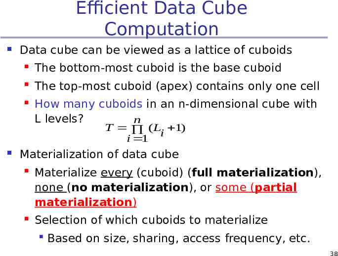
Efficient Data Cube Computation Data cube can be viewed as a lattice of cuboids The bottom-most cuboid is the base cuboid The top-most cuboid (apex) contains only one cell How many cuboids in an n-dimensional cube with L levels? n T ( Li 1) i 1 Materialization of data cube Materialize every (cuboid) (full materialization), none (no materialization), or some (partial materialization) Selection of which cuboids to materialize Based on size, sharing, access frequency, etc. 38
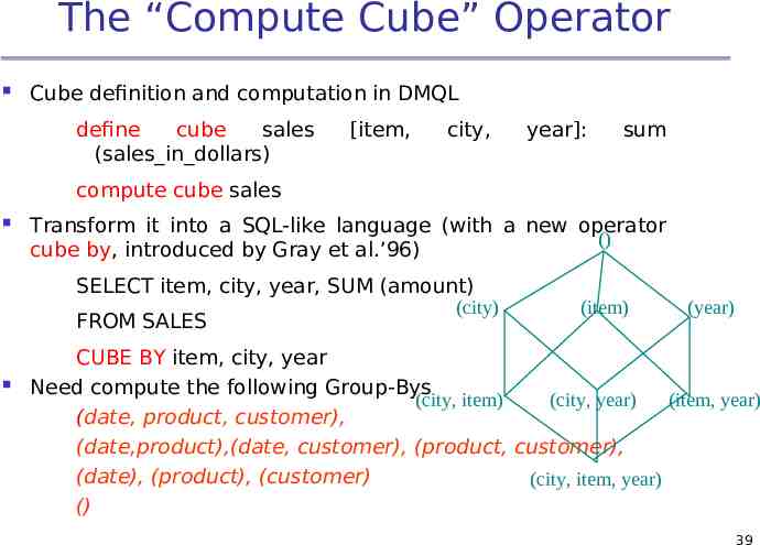
The “Compute Cube” Operator Cube definition and computation in DMQL define cube sales (sales in dollars) [item, city, year]: sum compute cube sales Transform it into a SQL-like language (with a new operator () cube by, introduced by Gray et al.’96) SELECT item, city, year, SUM (amount) (city) FROM SALES (item) (year) CUBE BY item, city, year Need compute the following Group-Bys (city, item) (city, year) (item, year) (date, product, customer), (date,product),(date, customer), (product, customer), (date), (product), (customer) (city, item, year) () 39
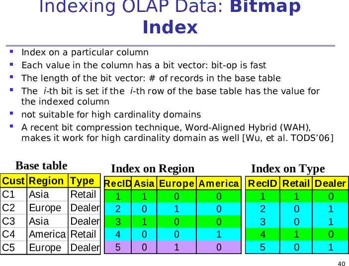
Indexing OLAP Data: Bitmap Index Index on a particular column Each value in the column has a bit vector: bit-op is fast The length of the bit vector: # of records in the base table The i-th bit is set if the i-th row of the base table has the value for the indexed column not suitable for high cardinality domains A recent bit compression technique, Word-Aligned Hybrid (WAH), makes it work for high cardinality domain as well [Wu, et al. TODS’06] Base table Cust C1 C2 C3 C4 C5 Region Asia Europe Asia America Europe Index on Region Index on Type Type RecID Asia Europe Am erica RecID Retail Dealer Retail 1 1 0 0 1 1 0 Dealer 2 0 1 0 2 0 1 Dealer 3 1 0 0 3 0 1 Retail 4 0 0 1 4 1 0 0 1 0 5 0 1 Dealer 5 40
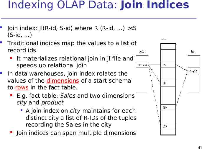
Indexing OLAP Data: Join Indices Join index: JI(R-id, S-id) where R (R-id, ) S (S-id, ) Traditional indices map the values to a list of record ids It materializes relational join in JI file and speeds up relational join In data warehouses, join index relates the values of the dimensions of a start schema to rows in the fact table. E.g. fact table: Sales and two dimensions city and product A join index on city maintains for each distinct city a list of R-IDs of the tuples recording the Sales in the city Join indices can span multiple dimensions 41
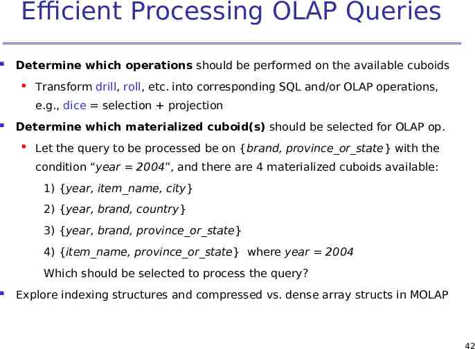
Efficient Processing OLAP Queries Determine which operations should be performed on the available cuboids Transform drill, roll, etc. into corresponding SQL and/or OLAP operations, e.g., dice selection projection Determine which materialized cuboid(s) should be selected for OLAP op. Let the query to be processed be on {brand, province or state} with the condition “year 2004”, and there are 4 materialized cuboids available: 1) {year, item name, city} 2) {year, brand, country} 3) {year, brand, province or state} 4) {item name, province or state} where year 2004 Which should be selected to process the query? Explore indexing structures and compressed vs. dense array structs in MOLAP 42
OLAP Server Architectures Relational OLAP (ROLAP) Use relational or extended-relational DBMS to store and manage warehouse data and OLAP middle ware Include optimization of DBMS backend, implementation of aggregation navigation logic, and additional tools and services Multidimensional OLAP (MOLAP) Sparse array-based multidimensional storage engine Fast indexing to pre-computed summarized data Hybrid OLAP (HOLAP) (e.g., Microsoft SQLServer) Greater scalability Flexibility, e.g., low level: relational, high-level: array Specialized SQL servers (e.g., Redbricks) Specialized support for SQL queries over star/snowflake schemas 43
Chapter 4: Data Warehousing and On-line Analytical Processing Data Warehouse: Basic Concepts Data Warehouse Modeling: Data Cube and OLAP Data Warehouse Design and Usage Data Warehouse Implementation Data Generalization by Attribute-Oriented Induction Summary 44
Attribute-Oriented Induction Proposed in 1989 (KDD ‘89 workshop) Not confined to categorical data nor particular measures How it is done? Collect the task-relevant data (initial relation) using a relational database query Perform generalization by attribute removal or attribute generalization Apply aggregation by merging identical, generalized tuples and accumulating their respective counts Interaction with users for knowledge presentation 45
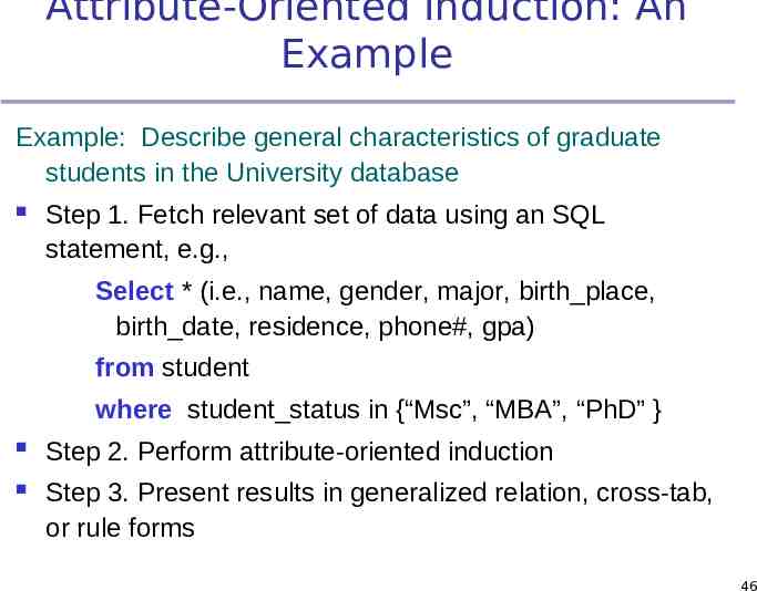
Attribute-Oriented Induction: An Example Example: Describe general characteristics of graduate students in the University database Step 1. Fetch relevant set of data using an SQL statement, e.g., Select * (i.e., name, gender, major, birth place, birth date, residence, phone#, gpa) from student where student status in {“Msc”, “MBA”, “PhD” } Step 2. Perform attribute-oriented induction Step 3. Present results in generalized relation, cross-tab, or rule forms 46
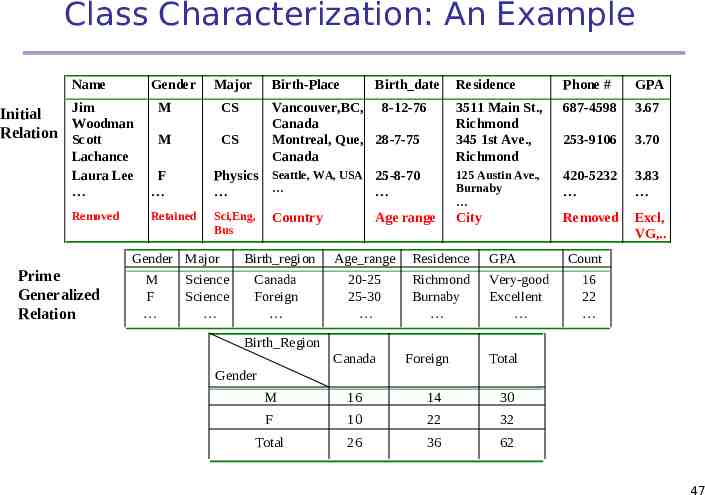
Class Characterization: An Example Name Gender Jim Initial Woodman Relation Scott M Major Vancouver,BC, 8-12-76 Canada CS Montreal, Que, 28-7-75 Canada Physics Seattle, WA, USA 25-8-70 M F Removed Retained Sci,Eng, Bus Gender Major M F Birth date CS Lachance Laura Lee Prime Generalized Relation Birth-Place Science Science Country Age range Residence Phone # GPA 3511 Main St., Richmond 345 1st Ave., Richmond 687-4598 3.67 253-9106 3.70 125 Austin Ave., Burnaby 420-5232 3.83 City Removed Excl, VG,. Birth region Age range Residence GPA Canada Foreign 20-25 25-30 Richmond Burnaby Very-good Excellent Count 16 22 Birth Region Canada Foreign Total Gender M 16 14 30 F 10 22 32 Total 26 36 62 47
Basic Principles of Attribute-Oriented Induction Data focusing: task-relevant data, including dimensions, and the result is the initial relation Attribute-removal: remove attribute A if there is a large set of distinct values for A but (1) there is no generalization operator on A, or (2) A’s higher level concepts are expressed in terms of other attributes Attribute-generalization: If there is a large set of distinct values for A, and there exists a set of generalization operators on A, then select an operator and generalize A Attribute-threshold control: typical 2-8, specified/default Generalized relation threshold control: control the final relation/rule size 48
Attribute-Oriented Induction: Basic Algorithm InitialRel: Query processing of task-relevant data, deriving the initial relation. PreGen: Based on the analysis of the number of distinct values in each attribute, determine generalization plan for each attribute: removal? or how high to generalize? PrimeGen: Based on the PreGen plan, perform generalization to the right level to derive a “prime generalized relation”, accumulating the counts. Presentation: User interaction: (1) adjust levels by drilling, (2) pivoting, (3) mapping into rules, cross tabs, visualization presentations. 49
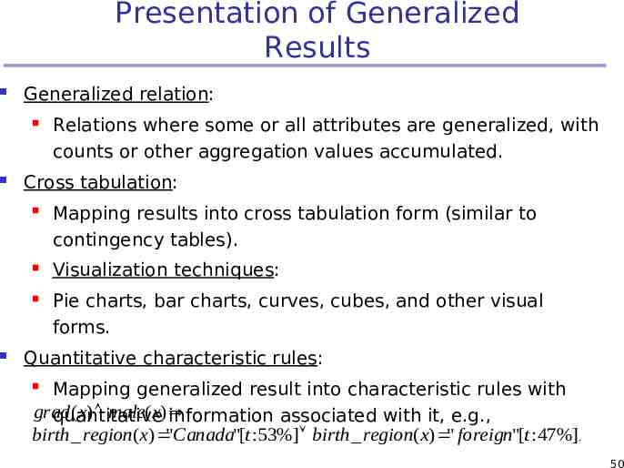
Presentation of Generalized Results Generalized relation: Cross tabulation: Relations where some or all attributes are generalized, with counts or other aggregation values accumulated. Mapping results into cross tabulation form (similar to contingency tables). Visualization techniques: Pie charts, bar charts, curves, cubes, and other visual forms. Quantitative characteristic rules: Mapping generalized result into characteristic rules with grad ( x) male( x) quantitative information associated with it, e.g., birth region( x) "Canada"[t :53%] birth region( x) " foreign"[t : 47%]. 50
Mining Class Comparisons Comparison: Comparing two or more classes Method: Partition the set of relevant data into the target class and the contrasting class(es) Generalize both classes to the same high level concepts Compare tuples with the same high level descriptions Present for every tuple its description and two measures support - distribution within single class comparison - distribution between classes Highlight the tuples with strong discriminant features Relevance Analysis: Find attributes (features) which best distinguish different classes 51
Concept Description vs. Cube-Based OLAP Similarity: Data generalization Presentation of data summarization at multiple levels of abstraction Interactive drilling, pivoting, slicing and dicing Differences: OLAP has systematic preprocessing, query independent, and can drill down to rather low level AOI has automated desired level allocation, and may perform dimension relevance analysis/ranking when there are many relevant dimensions AOI works on the data which are not in relational forms 52
Chapter 4: Data Warehousing and On-line Analytical Processing Data Warehouse: Basic Concepts Data Warehouse Modeling: Data Cube and OLAP Data Warehouse Design and Usage Data Warehouse Implementation Data Generalization by Attribute-Oriented Induction Summary 53
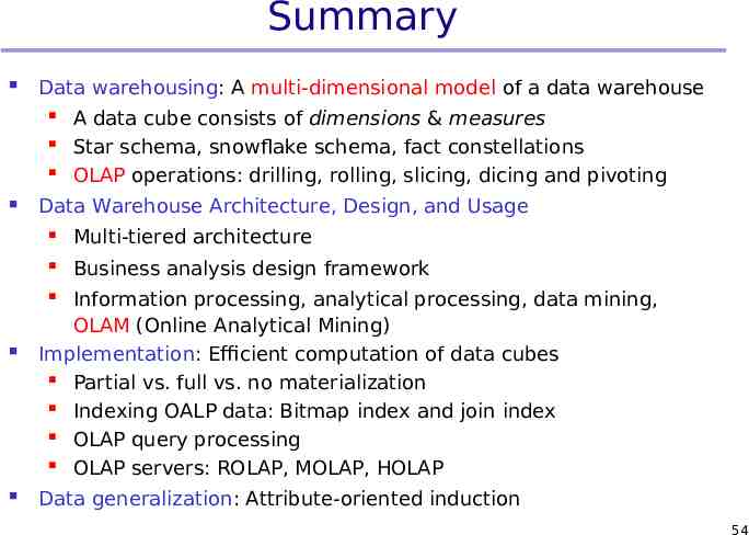
Summary Data warehousing: A multi-dimensional model of a data warehouse A data cube consists of dimensions & measures Star schema, snowflake schema, fact constellations OLAP operations: drilling, rolling, slicing, dicing and pivoting Data Warehouse Architecture, Design, and Usage Multi-tiered architecture Business analysis design framework Information processing, analytical processing, data mining, OLAM (Online Analytical Mining) Implementation: Efficient computation of data cubes Partial vs. full vs. no materialization Indexing OALP data: Bitmap index and join index OLAP query processing OLAP servers: ROLAP, MOLAP, HOLAP Data generalization: Attribute-oriented induction 54
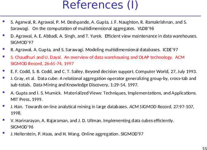
References (I) S. Agarwal, R. Agrawal, P. M. Deshpande, A. Gupta, J. F. Naughton, R. Ramakrishnan, and S. Sarawagi. On the computation of multidimensional aggregates. VLDB’96 D. Agrawal, A. E. Abbadi, A. Singh, and T. Yurek. Efficient view maintenance in data warehouses. SIGMOD’97 R. Agrawal, A. Gupta, and S. Sarawagi. Modeling multidimensional databases. ICDE’97 S. Chaudhuri and U. Dayal. An overview of data warehousing and OLAP technology. ACM SIGMOD Record, 26:65-74, 1997 E. F. Codd, S. B. Codd, and C. T. Salley. Beyond decision support. Computer World, 27, July 1993. J. Gray, et al. Data cube: A relational aggregation operator generalizing group-by, cross-tab and sub-totals. Data Mining and Knowledge Discovery, 1:29-54, 1997. A. Gupta and I. S. Mumick. Materialized Views: Techniques, Implementations, and Applications. MIT Press, 1999. J. Han. Towards on-line analytical mining in large databases. ACM SIGMOD Record, 27:97-107, 1998. V. Harinarayan, A. Rajaraman, and J. D. Ullman. Implementing data cubes efficiently. SIGMOD’96 J. Hellerstein, P. Haas, and H. Wang. Online aggregation. SIGMOD'97 55
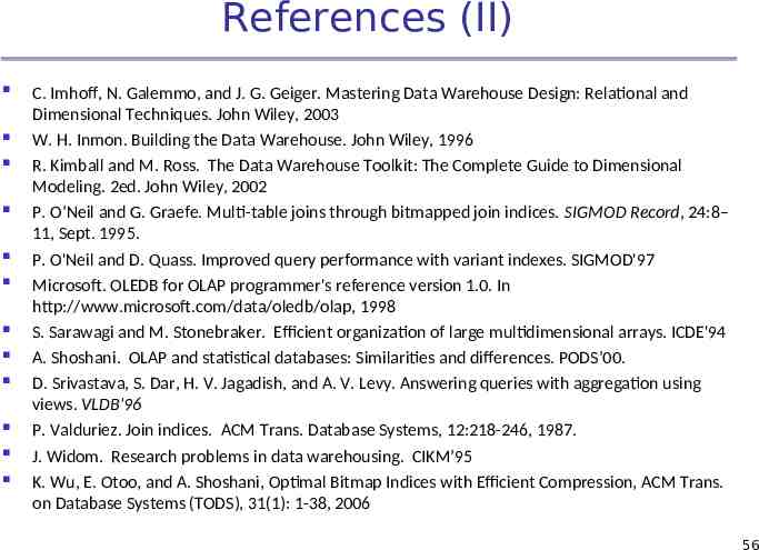
References (II) C. Imhoff, N. Galemmo, and J. G. Geiger. Mastering Data Warehouse Design: Relational and Dimensional Techniques. John Wiley, 2003 W. H. Inmon. Building the Data Warehouse. John Wiley, 1996 R. Kimball and M. Ross. The Data Warehouse Toolkit: The Complete Guide to Dimensional Modeling. 2ed. John Wiley, 2002 P. O’Neil and G. Graefe. Multi-table joins through bitmapped join indices. SIGMOD Record, 24:8– 11, Sept. 1995. P. O'Neil and D. Quass. Improved query performance with variant indexes. SIGMOD'97 Microsoft. OLEDB for OLAP programmer's reference version 1.0. In http://www.microsoft.com/data/oledb/olap, 1998 S. Sarawagi and M. Stonebraker. Efficient organization of large multidimensional arrays. ICDE'94 A. Shoshani. OLAP and statistical databases: Similarities and differences. PODS’00. D. Srivastava, S. Dar, H. V. Jagadish, and A. V. Levy. Answering queries with aggregation using views. VLDB'96 P. Valduriez. Join indices. ACM Trans. Database Systems, 12:218-246, 1987. J. Widom. Research problems in data warehousing. CIKM’95 K. Wu, E. Otoo, and A. Shoshani, Optimal Bitmap Indices with Efficient Compression, ACM Trans. on Database Systems (TODS), 31(1): 1-38, 2006 56
Surplus Slides 57
Compression of Bitmap Indices Bitmap indexes must be compressed to reduce I/O costs and minimize CPU usage—majority of the bits are 0’s Two compression schemes: Byte-aligned Bitmap Code (BBC) Word-Aligned Hybrid (WAH) code Time and space required to operate on compressed bitmap is proportional to the total size of the bitmap Optimal on attributes of low cardinality as well as those of high cardinality. WAH out performs BBC by about a factor of two 58