CS490D: Introduction to Data Mining Prof. Chris Clifton March 12,


64 Slides894.50 KB
CS490D: Introduction to Data Mining Prof. Chris Clifton March 12, 2004 Data Mining Process
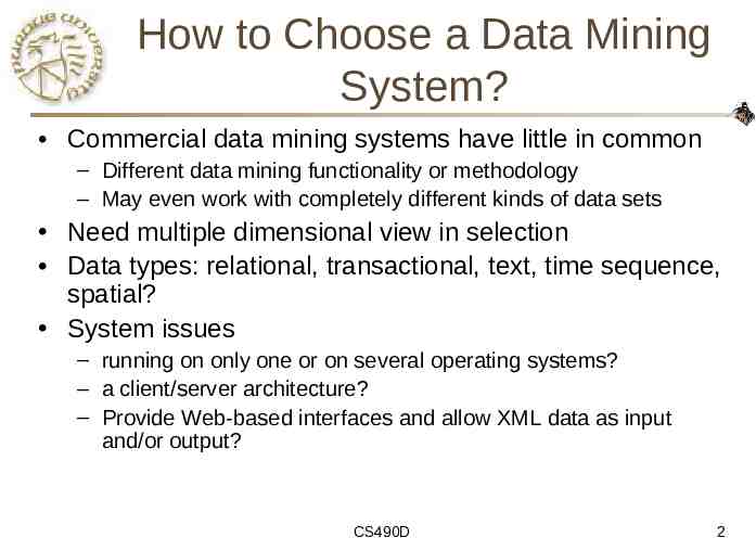
How to Choose a Data Mining System? Commercial data mining systems have little in common – Different data mining functionality or methodology – May even work with completely different kinds of data sets Need multiple dimensional view in selection Data types: relational, transactional, text, time sequence, spatial? System issues – running on only one or on several operating systems? – a client/server architecture? – Provide Web-based interfaces and allow XML data as input and/or output? CS490D 2
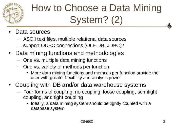
How to Choose a Data Mining System? (2) Data sources – ASCII text files, multiple relational data sources – support ODBC connections (OLE DB, JDBC)? Data mining functions and methodologies – One vs. multiple data mining functions – One vs. variety of methods per function More data mining functions and methods per function provide the user with greater flexibility and analysis power Coupling with DB and/or data warehouse systems – Four forms of coupling: no coupling, loose coupling, semitight coupling, and tight coupling Ideally, a data mining system should be tightly coupled with a database system CS490D 3
How to Choose a Data Mining System? (3) Scalability – Row (or database size) scalability – Column (or dimension) scalability – Curse of dimensionality: it is much more challenging to make a system column scalable that row scalable Visualization tools – “A picture is worth a thousand words” – Visualization categories: data visualization, mining result visualization, mining process visualization, and visual data mining Data mining query language and graphical user interface – Easy-to-use and high-quality graphical user interface – Essential for user-guided, highly interactive data mining CS490D 4
Examples of Data Mining Systems (1) IBM Intelligent Miner – A wide range of data mining algorithms – Scalable mining algorithms – Toolkits: neural network algorithms, statistical methods, data preparation, and data visualization tools – Tight integration with IBM's DB2 relational database system SAS Enterprise Miner – A variety of statistical analysis tools – Data warehouse tools and multiple data mining algorithms Mirosoft SQLServer 2000 – Integrate DB and OLAP with mining – Support OLEDB for DM standard CS490D 5
Examples of Data Mining Systems (2) SGI MineSet – Multiple data mining algorithms and advanced statistics – Advanced visualization tools Clementine (SPSS) – An integrated data mining development environment for endusers and developers – Multiple data mining algorithms and visualization tools DBMiner (DBMiner Technology Inc.) – Multiple data mining modules: discovery-driven OLAP analysis, association, classification, and clustering – Efficient, association and sequential-pattern mining functions, and visual classification tool – Mining both relational databases and data warehouses CS490D 6
CS490D: Introduction to Data Mining Prof. Chris Clifton March 22, 2004 CRISP-DM Thanks to Laura Squier, SPSS for some of the material used
SIGMOD’04 Scholarships Want to learn more about Database and Data Mining Research? – SIGMOD is the premier database research conference Want 1000 off a trip to France this summer? – June 13-18, Paris Application Deadline March 26 – Details: http://www.cs.rpi.edu/sigmod-ugrad CS490D 8
CS490D: Introduction to Data Mining Prof. Chris Clifton March 22, 2004 CRISP-DM Thanks to Laura Squier, SPSS for some of the material used
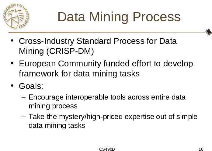
Data Mining Process Cross-Industry Standard Process for Data Mining (CRISP-DM) European Community funded effort to develop framework for data mining tasks Goals: – Encourage interoperable tools across entire data mining process – Take the mystery/high-priced expertise out of simple data mining tasks CS490D 10
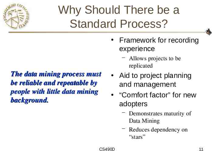
Why Should There be a Standard Process? Framework for recording experience – Allows projects to be replicated The data mining process must be reliable and repeatable by people with little data mining background. Aid to project planning and management “Comfort factor” for new adopters – Demonstrates maturity of Data Mining – Reduces dependency on “stars” CS490D 11
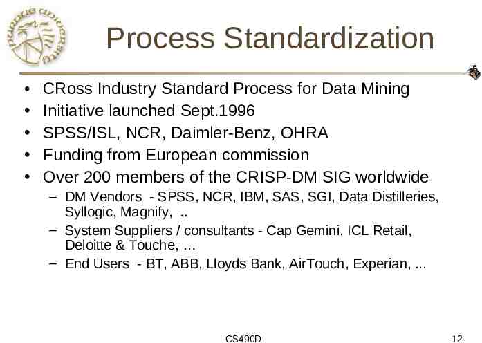
Process Standardization CRoss Industry Standard Process for Data Mining Initiative launched Sept.1996 SPSS/ISL, NCR, Daimler-Benz, OHRA Funding from European commission Over 200 members of the CRISP-DM SIG worldwide – DM Vendors - SPSS, NCR, IBM, SAS, SGI, Data Distilleries, Syllogic, Magnify, . – System Suppliers / consultants - Cap Gemini, ICL Retail, Deloitte & Touche, – End Users - BT, ABB, Lloyds Bank, AirTouch, Experian, . CS490D 12
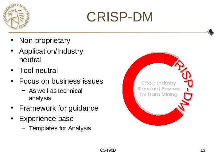
CRISP-DM Non-proprietary Application/Industry neutral Tool neutral Focus on business issues – As well as technical analysis Framework for guidance Experience base – Templates for Analysis CS490D 13
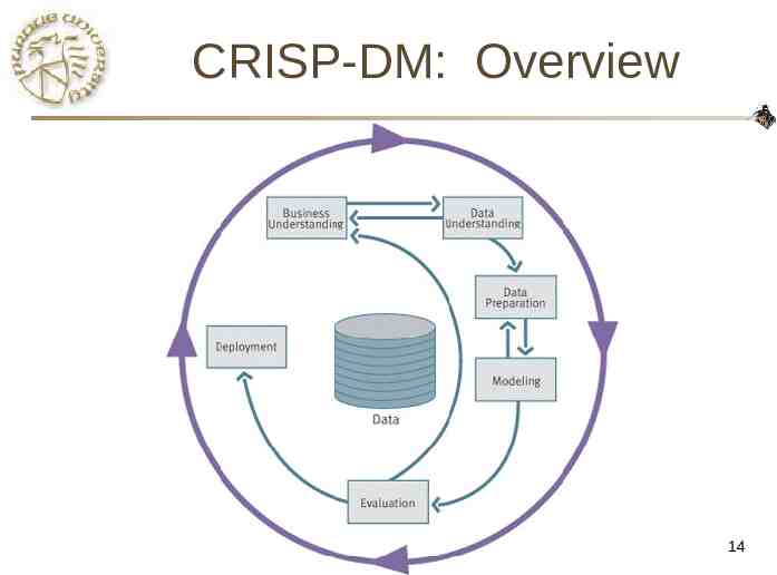
CRISP-DM: Overview CS490D 14
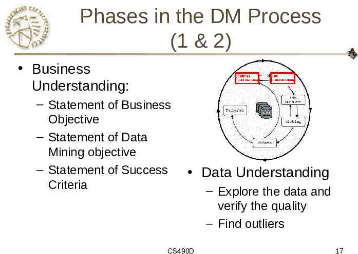
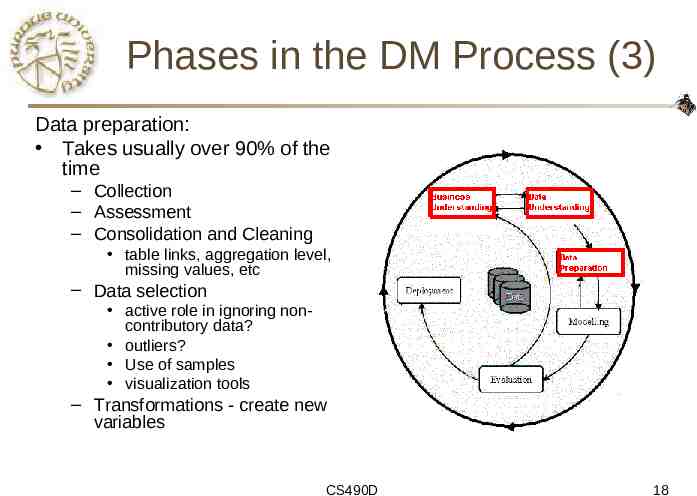
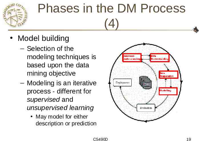
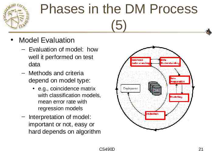
CRISP-DM: Phases Business Understanding – – Data Understanding – – – Run the data mining tools Evaluation – – Record and attribute selection Data cleansing Modeling – Initial data collection and familiarization Identify data quality issues Initial, obvious results Data Preparation – – Understanding project objectives and requirements Data mining problem definition Determine if results meet business objectives Identify business issues that should have been addressed earlier Deployment – – Put the resulting models into practice Set up for repeated/continuous mining of the data CS490D 15
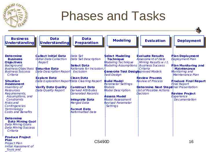
Phases and Tasks Business Understanding Determine Business Objectives Background Business Objectives Business Success Criteria Situation Assessment Inventory of Resources Requirements, Assumptions, and Constraints Risks and Contingencies Terminology Costs and Benefits Data Understanding Collect Initial Data Initial Data Collection Report Data Preparation Modeling Evaluation Deployment Data Set Data Set Description Select Modeling Evaluate Results Plan Deployment Technique Assessment of Data Deployment Plan Modeling Technique Mining Results w.r.t. Select Data Modeling Assumptions Business Success Plan Monitoring and Describe Data Rationale for Inclusion / Criteria Maintenance Data Description Report Exclusion Generate Test Design Approved Models Monitoring and Test Design Maintenance Plan Explore Data Clean Data Review Process Data Exploration ReportData Cleaning Report Build Model Review of Process Produce Final Report Parameter Settings Final Report Verify Data Quality Construct Data Models Determine Next StepsFinal Presentation Data Quality Report Derived Attributes Model Description List of Possible Actions Generated Records Decision Review Project Assess Model Experience Integrate Data Model Assessment Documentation Merged Data Revised Parameter Settings Format Data Reformatted Data Determine Data Mining Goal Data Mining Goals Data Mining Success Criteria Produce Project Plan Project Plan Initial Asessment of Tools and CS490D 16
Phases in the DM Process (1 & 2) Business Understanding: – Statement of Business Objective – Statement of Data Mining objective – Statement of Success Criteria Data Understanding CS490D – Explore the data and verify the quality – Find outliers 17
Phases in the DM Process (3) Data preparation: Takes usually over 90% of the time – Collection – Assessment – Consolidation and Cleaning table links, aggregation level, missing values, etc – Data selection active role in ignoring noncontributory data? outliers? Use of samples visualization tools – Transformations - create new variables CS490D 18
Phases in the DM Process (4) Model building – Selection of the modeling techniques is based upon the data mining objective – Modeling is an iterative process - different for supervised and unsupervised learning May model for either description or prediction CS490D 19
Phases in the DM Process (5) Model Evaluation – Evaluation of model: how well it performed on test data – Methods and criteria depend on model type: e.g., coincidence matrix with classification models, mean error rate with regression models – Interpretation of model: important or not, easy or hard depends on algorithm CS490D 21
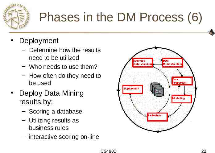
Phases in the DM Process (6) Deployment – Determine how the results need to be utilized – Who needs to use them? – How often do they need to be used Deploy Data Mining results by: – Scoring a database – Utilizing results as business rules – interactive scoring on-line CS490D 22
Why CRISP-DM? The data mining process must be reliable and repeatable by people with little data mining skills CRISP-DM provides a uniform framework for – guidelines – experience documentation CRISP-DM is flexible to account for differences – Different business/agency problems – Different data CS490D 23
CS490D: Introduction to Data Mining Prof. Chris Clifton March 24, 2004 Attribute-Oriented Induction
Attribute-Oriented Induction Proposed in 1989 (KDD ‘89 workshop) Not confined to categorical data nor particular measures. How it is done? – Collect the task-relevant data (initial relation) using a relational database query – Perform generalization by attribute removal or attribute generalization. – Apply aggregation by merging identical, generalized tuples and accumulating their respective counts – Interactive presentation with users CS490D 32
Basic Principles of AttributeOriented Induction Data focusing: task-relevant data, including dimensions, and the result is the initial relation. Attribute-removal: remove attribute A if there is a large set of distinct values for A but (1) there is no generalization operator on A, or (2) A’s higher level concepts are expressed in terms of other attributes. Attribute-generalization: If there is a large set of distinct values for A, and there exists a set of generalization operators on A, then select an operator and generalize A. Attribute-threshold control: typical 2-8, specified/default. Generalized relation threshold control: control the final relation/rule size. see example May 4, 2023 CS490D
Attribute-Oriented Induction: Basic Algorithm InitialRel: Query processing of task-relevant data, deriving the initial relation. PreGen: Based on the analysis of the number of distinct values in each attribute, determine generalization plan for each attribute: removal? or how high to generalize? PrimeGen: Based on the PreGen plan, perform generalization to the right level to derive a “prime generalized relation”, accumulating the counts. Presentation: User interaction: (1) adjust levels by drilling, (2) pivoting, (3) mapping into rules, cross tabs, visualization presentations. May 4, 2023 CS490D
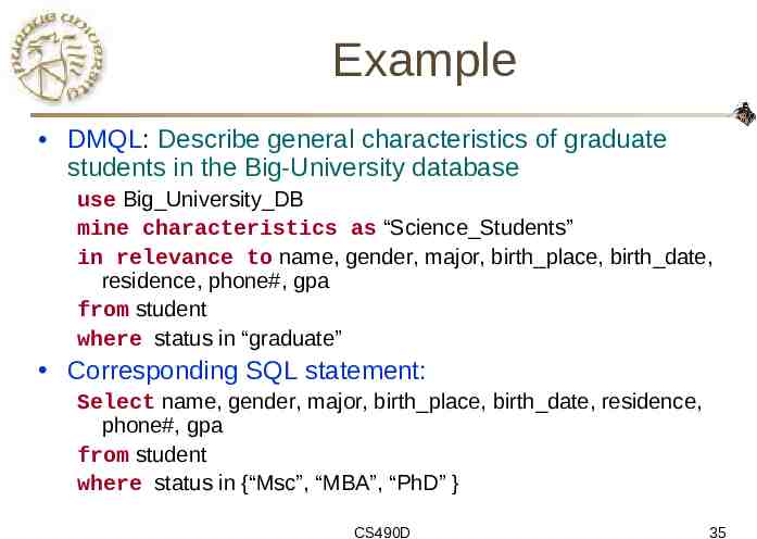
Example DMQL: Describe general characteristics of graduate students in the Big-University database use Big University DB mine characteristics as “Science Students” in relevance to name, gender, major, birth place, birth date, residence, phone#, gpa from student where status in “graduate” Corresponding SQL statement: Select name, gender, major, birth place, birth date, residence, phone#, gpa from student where status in {“Msc”, “MBA”, “PhD” } CS490D 35
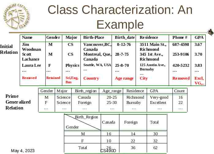
Class Characterization: An Example Name Gender Jim Initial Woodman Relation Scott M Major M F Removed Retained Residence Phone # GPA Vancouver,BC, 8-12-76 Canada CS Montreal, Que, 28-7-75 Canada Physics Seattle, WA, USA 25-8-70 3511 Main St., Richmond 345 1st Ave., Richmond 687-4598 3.67 253-9106 3.70 125 Austin Ave., Burnaby 420-5232 3.83 Sci,Eng, Bus City Removed Excl, VG,. Gender Major M F Birth date CS Lachance Laura Lee Prime Generalized Relation Birth-Place Science Science Country Age range Birth region Age range Residence GPA Canada Foreign 20-25 25-30 Richmond Burnaby Very-good Excellent Birth Region Canada Foreign Total Gender May 4, 2023 M 16 14 30 F 10 22 32 Total 26 CS490D 36 62 Count 16 22
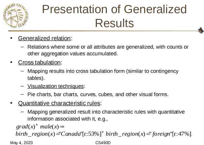
Presentation of Generalized Results Generalized relation: – Relations where some or all attributes are generalized, with counts or other aggregation values accumulated. Cross tabulation: – Mapping results into cross tabulation form (similar to contingency tables). – Visualization techniques: – Pie charts, bar charts, curves, cubes, and other visual forms. Quantitative characteristic rules: – Mapping generalized result into characteristic rules with quantitative information associated with it, e.g., grad ( x) male( x) birth region( x) "Canada"[t :53%] birth region( x) " foreign"[t : 47%]. May 4, 2023 CS490D
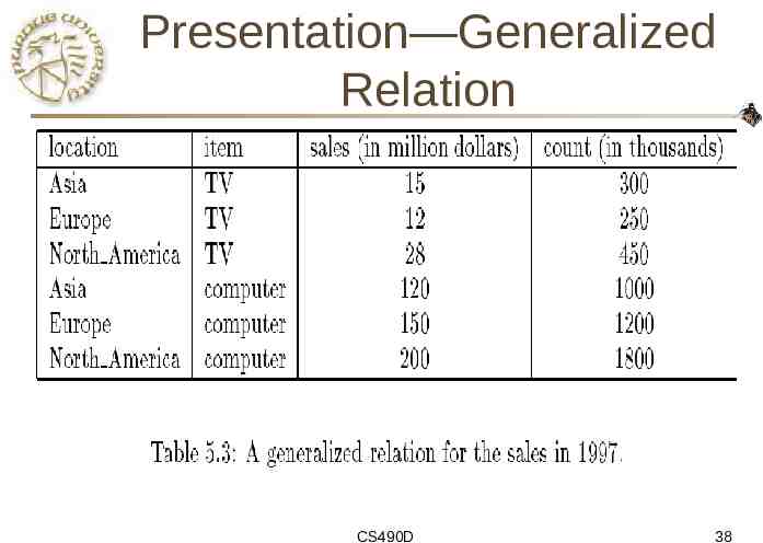
Presentation—Generalized Relation CS490D 38
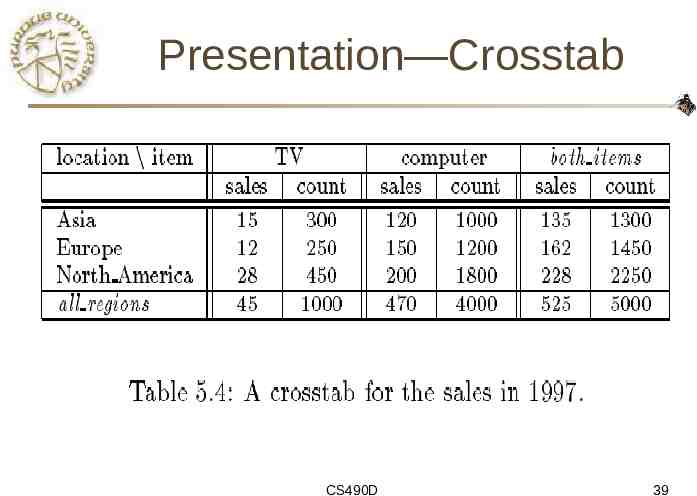
Presentation—Crosstab CS490D 39
Concept Description: Characterization and Comparison What is concept description? Data generalization and summarization-based characterization Analytical characterization: Analysis of attribute relevance Mining class comparisons: Discriminating between different classes Mining descriptive statistical measures in large databases Discussion Summary CS490D 41
Characterization vs. OLAP Similarity: – Presentation of data summarization at multiple levels of abstraction. – Interactive drilling, pivoting, slicing and dicing. Differences: – Automated desired level allocation. – Dimension relevance analysis and ranking when there are many relevant dimensions. – Sophisticated typing on dimensions and measures. – Analytical characterization: data dispersion analysis. CS490D 42
Attribute Relevance Analysis Why? – – – – Which dimensions should be included? How high level of generalization? Automatic VS. Interactive Reduce # attributes; Easy to understand patterns What? – statistical method for preprocessing data filter out irrelevant or weakly relevant attributes retain or rank the relevant attributes – relevance related to dimensions and levels – analytical characterization, analytical comparison CS490D 43
Attribute relevance analysis (cont’d) How? – Data Collection – Analytical Generalization Use information gain analysis (e.g., entropy or other measures) to identify highly relevant dimensions and levels. – Relevance Analysis Sort and select the most relevant dimensions and levels. – Attribute-oriented Induction for class description On selected dimension/level – OLAP operations (e.g. drilling, slicing) on relevance rules CS490D 44
Relevance Measures Quantitative relevance measure determines the classifying power of an attribute within a set of data. Methods – information gain (ID3) – gain ratio (C4.5) – gini index 2 contingency table statistics – uncertainty coefficient CS490D 45
Information-Theoretic Approach Decision tree – each internal node tests an attribute – each branch corresponds to attribute value – each leaf node assigns a classification ID3 algorithm – build decision tree based on training objects with known class labels to classify testing objects – rank attributes with information gain measure – minimal height the least number of tests to classify an object CS490D 46
Example: Analytical Characterization Task – Mine general characteristics describing graduate students using analytical characterization Given – attributes name, gender, major, birth place, birth date, phone#, and gpa – Gen(ai) concept hierarchies on ai – Ui attribute analytical thresholds for ai – Ti attribute generalization thresholds for ai – R attribute relevance threshold CS490D 49
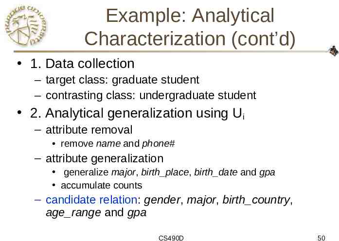
Example: Analytical Characterization (cont’d) 1. Data collection – target class: graduate student – contrasting class: undergraduate student 2. Analytical generalization using Ui – attribute removal remove name and phone# – attribute generalization generalize major, birth place, birth date and gpa accumulate counts – candidate relation: gender, major, birth country, age range and gpa CS490D 50
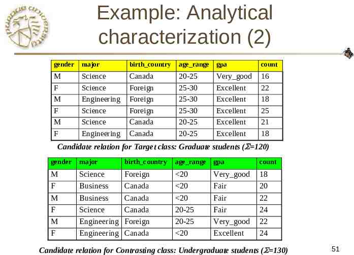
Example: Analytical characterization (2) gender major birth country age range gpa count M F M F M F Science Science Engineering Science Science Engineering Canada Foreign Foreign Foreign Canada Canada 20-25 25-30 25-30 25-30 20-25 20-25 Very good Excellent Excellent Excellent Excellent Excellent 16 22 18 25 21 18 Candidate relation for Target class: Graduate students ( 120) gender major birth country age range gpa count M F M F M F Science Business Business Science Engineering Engineering Foreign Canada Canada Canada Foreign Canada 20 20 20 20-25 20-25 20 Very good Fair Fair Fair Very good Excellent 18 20 22 24 22 24 Candidate relation for Contrasting class: Undergraduate students ( 130) 51
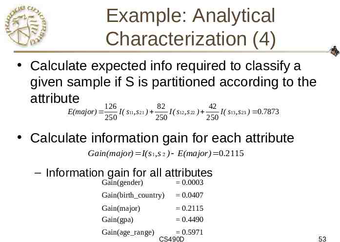
Example: Analytical characterization (3) 3. Relevance analysis – Calculate expected info required to classify an arbitrary tuple I(s 1, s 2 ) I( 120 ,130 ) 120 120 130 130 log 2 log 2 0.9988 250 250 250 250 – Calculate entropy of each attribute: e.g. major For major ”Science”: S11 84 S21 42 I(s11,s21) 0.9183 For major ”Engineering”: S12 36 S22 46 I(s12,s22) 0.9892 For major ”Business”: S23 42 I(s13,s23) 0 S13 0 Number of grad students in “Science” CS490D Number of undergrad students in “Science” 52
Example: Analytical Characterization (4) Calculate expected info required to classify a given sample if S is partitioned according to the attribute 126 82 42 E(major) 250 I ( s11, s 21 ) 250 I ( s12 , s 22 ) 250 I ( s13, s 23 ) 0.7873 Calculate information gain for each attribute Gain(major) I(s 1, s 2 ) E(major) 0.2115 – Information gain for all attributes Gain(gender) 0.0003 Gain(birth country) 0.0407 Gain(major) Gain(gpa) 0.2115 0.4490 Gain(age range) 0.5971 CS490D 53
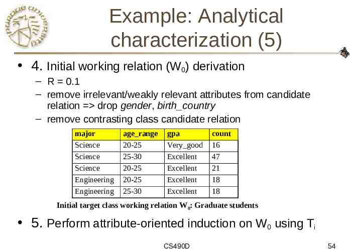
Example: Analytical characterization (5) 4. Initial working relation (W0) derivation – R 0.1 – remove irrelevant/weakly relevant attributes from candidate relation drop gender, birth country – remove contrasting class candidate relation major Science Science Science Engineering Engineering age range 20-25 25-30 20-25 20-25 25-30 gpa Very good Excellent Excellent Excellent Excellent count 16 47 21 18 18 Initial target class working relation W0: Graduate students 5. Perform attribute-oriented induction on W0 using Ti CS490D 54
Concept Description: Characterization and Comparison What is concept description? Data generalization and summarization-based characterization Analytical characterization: Analysis of attribute relevance Mining class comparisons: Discriminating between different classes Mining descriptive statistical measures in large databases Discussion Summary CS490D 55
Mining Class Comparisons Comparison: Comparing two or more classes Method: – Partition the set of relevant data into the target class and the contrasting class(es) – Generalize both classes to the same high level concepts – Compare tuples with the same high level descriptions – Present for every tuple its description and two measures – support - distribution within single class comparison - distribution between classes Highlight the tuples with strong discriminant features Relevance Analysis: – Find attributes (features) which best distinguish different classes May 4, 2023 CS490D
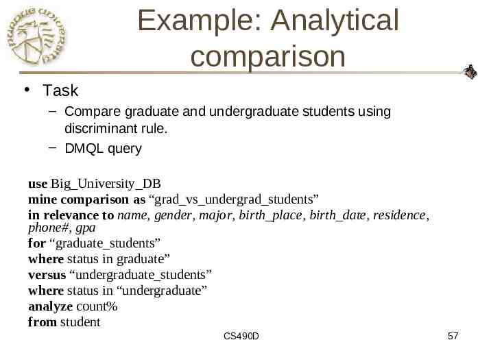
Example: Analytical comparison Task – Compare graduate and undergraduate students using discriminant rule. – DMQL query use Big University DB mine comparison as “grad vs undergrad students” in relevance to name, gender, major, birth place, birth date, residence, phone#, gpa for “graduate students” where status in graduate” versus “undergraduate students” where status in “undergraduate” analyze count% from student CS490D 57
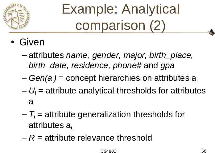
Example: Analytical comparison (2) Given – attributes name, gender, major, birth place, birth date, residence, phone# and gpa – Gen(ai) concept hierarchies on attributes ai – Ui attribute analytical thresholds for attributes ai – Ti attribute generalization thresholds for attributes ai – R attribute relevance threshold CS490D 58
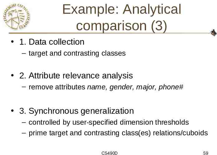
Example: Analytical comparison (3) 1. Data collection – target and contrasting classes 2. Attribute relevance analysis – remove attributes name, gender, major, phone# 3. Synchronous generalization – controlled by user-specified dimension thresholds – prime target and contrasting class(es) relations/cuboids CS490D 59
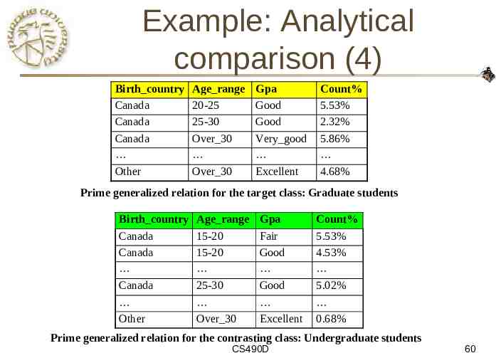
Example: Analytical comparison (4) Birth country Canada Canada Canada Other Age range 20-25 25-30 Over 30 Over 30 Gpa Good Good Very good Excellent Count% 5.53% 2.32% 5.86% 4.68% Prime generalized relation for the target class: Graduate students Birth country Canada Canada Canada Other Age range 15-20 15-20 25-30 Over 30 Gpa Fair Good Good Excellent Count% 5.53% 4.53% 5.02% 0.68% Prime generalized relation for the contrasting class: Undergraduate students CS490D 60
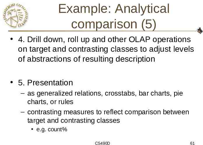
Example: Analytical comparison (5) 4. Drill down, roll up and other OLAP operations on target and contrasting classes to adjust levels of abstractions of resulting description 5. Presentation – as generalized relations, crosstabs, bar charts, pie charts, or rules – contrasting measures to reflect comparison between target and contrasting classes e.g. count% CS490D 61
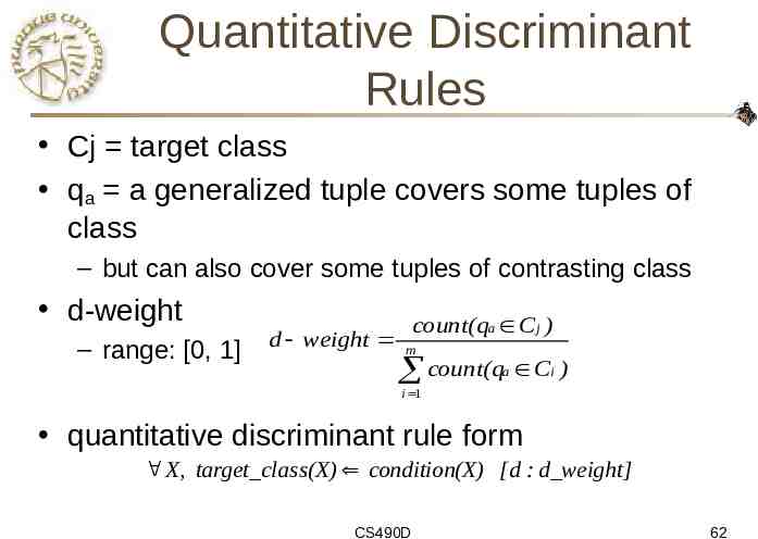
Quantitative Discriminant Rules Cj target class qa a generalized tuple covers some tuples of class – but can also cover some tuples of contrasting class d-weight – range: [0, 1] d weight count(qa Cj ) m count(q a Ci ) i 1 quantitative discriminant rule form X, target cla ss(X) condition(X) [d : d weight] CS490D 62
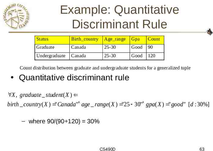
Example: Quantitative Discriminant Rule Status Birth country Age range Gpa Count Graduate Canada 25-30 Good 90 Undergraduate Canada 25-30 Good 120 Count distribution between graduate and undergraduate students for a generalized tuple Quantitative discriminant rule X , graduate student ( X ) birth country( X ) " Canada" age range( X ) "25 30" gpa( X ) " good" [d : 30%] – where 90/(90 120) 30% CS490D 63
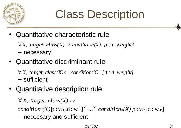
Class Description Quantitative characteristic rule X, target class(X) condition(X) [t : t weight] – necessary Quantitative discriminant rule X, target cla ss(X) condition(X) [d : d weight] – sufficient Quantitative description rule X, target class(X) condition 1(X) [t : w1, d : w 1] . conditionn(X) [t : wn, d : w n] – necessary and sufficient CS490D 64
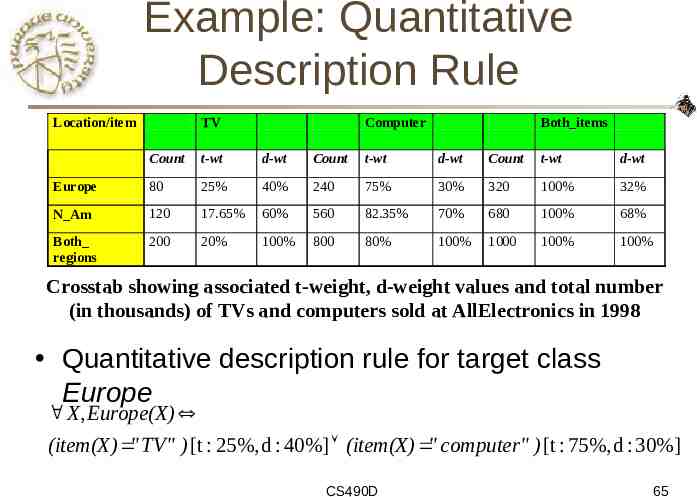
Example: Quantitative Description Rule Location/item TV Computer Both items Count t-wt d-wt Count t-wt d-wt Count t-wt d-wt Europe 80 25% 40% 240 75% 30% 320 100% 32% N Am 120 17.65% 60% 560 82.35% 70% 680 100% 68% Both regions 200 20% 100% 800 80% 100% 1000 100% 100% Crosstab showing associated t-weight, d-weight values and total number (in thousands) of TVs and computers sold at AllElectronics in 1998 Quantitative description rule for target class Europe X, Europe(X) (item(X) " TV" ) [t : 25%, d : 40%] (item(X) " computer" ) [t : 75%, d : 30%] CS490D 65
Concept Description: Characterization and Comparison What is concept description? Data generalization and summarization-based characterization Analytical characterization: Analysis of attribute relevance Mining class comparisons: Discriminating between different classes Mining descriptive statistical measures in large databases Discussion Summary CS490D 75
Mining Data Dispersion Characteristics Motivation – Data dispersion characteristics – To better understand the data: central tendency, variation and spread median, max, min, quantiles, outliers, variance, etc. Numerical dimensions correspond to sorted intervals – Data dispersion: analyzed with multiple granularities of precision – Boxplot or quantile analysis on sorted intervals Dispersion analysis on computed measures – Folding measures into numerical dimensions – Boxplot or quantile analysis on the transformed cube CS490D 76
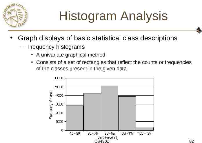
Histogram Analysis Graph displays of basic statistical class descriptions – Frequency histograms A univariate graphical method Consists of a set of rectangles that reflect the counts or frequencies of the classes present in the given data CS490D 82
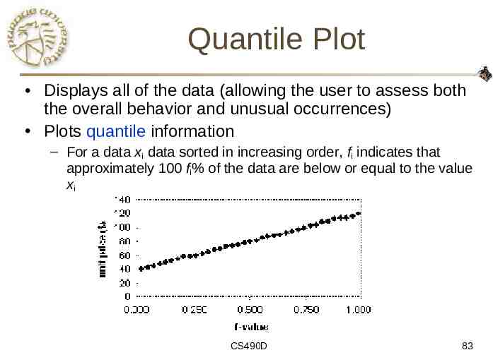
Quantile Plot Displays all of the data (allowing the user to assess both the overall behavior and unusual occurrences) Plots quantile information – For a data xi data sorted in increasing order, fi indicates that approximately 100 fi% of the data are below or equal to the value xi CS490D 83
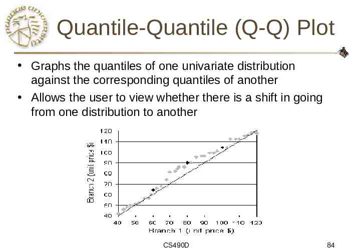
Quantile-Quantile (Q-Q) Plot Graphs the quantiles of one univariate distribution against the corresponding quantiles of another Allows the user to view whether there is a shift in going from one distribution to another CS490D 84
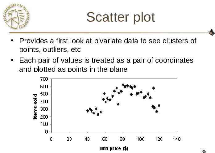
Scatter plot Provides a first look at bivariate data to see clusters of points, outliers, etc Each pair of values is treated as a pair of coordinates and plotted as points in the plane CS490D 85
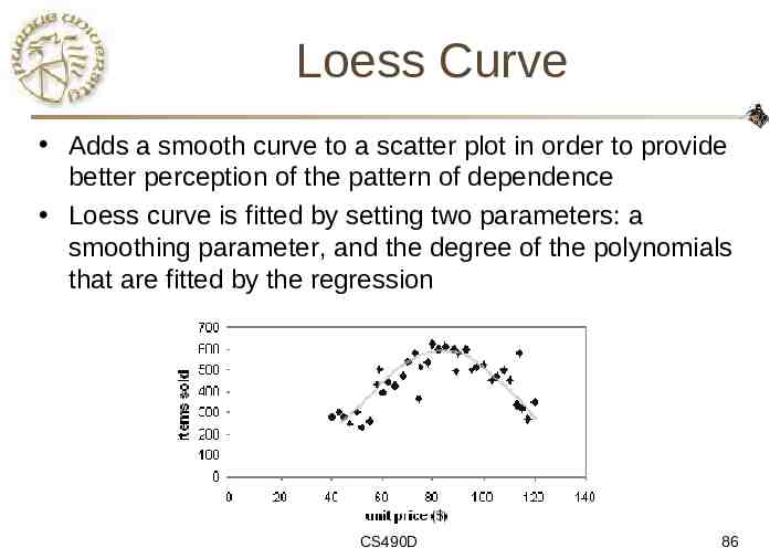
Loess Curve Adds a smooth curve to a scatter plot in order to provide better perception of the pattern of dependence Loess curve is fitted by setting two parameters: a smoothing parameter, and the degree of the polynomials that are fitted by the regression CS490D 86
Summary Concept description: characterization and discrimination OLAP-based vs. attribute-oriented induction Efficient implementation of AOI Analytical characterization and comparison Mining descriptive statistical measures in large databases Discussion – Incremental and parallel mining of description – Descriptive mining of complex types of data CS490D 93
References Y. Cai, N. Cercone, and J. Han. Attribute-oriented induction in relational databases. In G. Piatetsky-Shapiro and W. J. Frawley, editors, Knowledge Discovery in Databases, pages 213-228. AAAI/MIT Press, 1991. S. Chaudhuri and U. Dayal. An overview of data warehousing and OLAP technology. ACM SIGMOD Record, 26:65-74, 1997 C. Carter and H. Hamilton. Efficient attribute-oriented generalization for knowledge discovery from large databases. IEEE Trans. Knowledge and Data Engineering, 10:193-208, 1998. W. Cleveland. Visualizing Data. Hobart Press, Summit NJ, 1993. J. L. Devore. Probability and Statistics for Engineering and the Science, 4th ed. Duxbury Press, 1995. T. G. Dietterich and R. S. Michalski. A comparative review of selected methods for learning from examples. In Michalski et al., editor, Machine Learning: An Artificial Intelligence Approach, Vol. 1, pages 41-82. Morgan Kaufmann, 1983. J. Gray, S. Chaudhuri, A. Bosworth, A. Layman, D. Reichart, M. Venkatrao, F. Pellow, and H. Pirahesh. Data cube: A relational aggregation operator generalizing group-by, cross-tab and sub-totals. Data Mining and Knowledge Discovery, 1:29-54, 1997. J. Han, Y. Cai, and N. Cercone. Data-driven discovery of quantitative rules in relational databases. IEEE Trans. Knowledge and Data Engineering, 5:29-40, 1993. CS490D 94
References (cont.) J. Han and Y. Fu. Exploration of the power of attribute-oriented induction in data mining. In U.M. Fayyad, G. Piatetsky-Shapiro, P. Smyth, and R. Uthurusamy, editors, Advances in Knowledge Discovery and Data Mining, pages 399-421. AAAI/MIT Press, 1996. R. A. Johnson and D. A. Wichern. Applied Multivariate Statistical Analysis, 3rd ed. Prentice Hall, 1992. E. Knorr and R. Ng. Algorithms for mining distance-based outliers in large datasets. VLDB'98, New York, NY, Aug. 1998. H. Liu and H. Motoda. Feature Selection for Knowledge Discovery and Data Mining. Kluwer Academic Publishers, 1998. R. S. Michalski. A theory and methodology of inductive learning. In Michalski et al., editor, Machine Learning: An Artificial Intelligence Approach, Vol. 1, Morgan Kaufmann, 1983. T. M. Mitchell. Version spaces: A candidate elimination approach to rule learning. IJCAI'97, Cambridge, MA. T. M. Mitchell. Generalization as search. Artificial Intelligence, 18:203-226, 1982. T. M. Mitchell. Machine Learning. McGraw Hill, 1997. J. R. Quinlan. Induction of decision trees. Machine Learning, 1:81-106, 1986. D. Subramanian and J. Feigenbaum. Factorization in experiment generation. AAAI'86, Philadelphia, PA, Aug. 1986. CS490D 95