Business Intelligence and Data Analytics Intro Qiang Yang Based

24 Slides309.50 KB
Business Intelligence and Data Analytics Intro Qiang Yang Based on Textbook: Business Intelligence by Carlos Vercellis 1
Also adapted from sources Tan, Steinbach, Kumar (TSK) Book: Weka Book: Witten and Frank (WF): Data Mining Han and Kamber (HK Book): Introduction to Data Mining Data Mining BI Book is denoted as “BI Chapter #.” 2
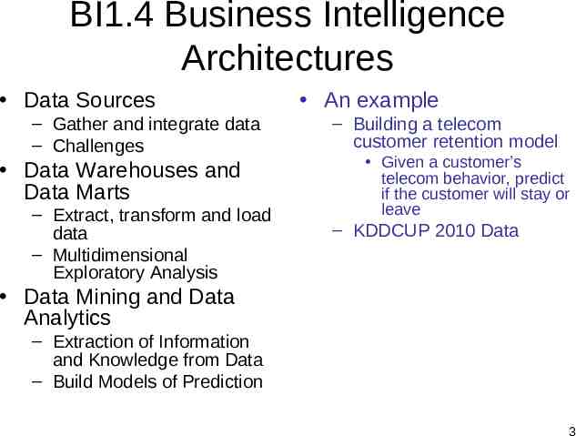
BI1.4 Business Intelligence Architectures Data Sources – Gather and integrate data – Challenges Data Warehouses and Data Marts – Extract, transform and load data – Multidimensional Exploratory Analysis An example – Building a telecom customer retention model Given a customer’s telecom behavior, predict if the customer will stay or leave – KDDCUP 2010 Data Data Mining and Data Analytics – Extraction of Information and Knowledge from Data – Build Models of Prediction 3
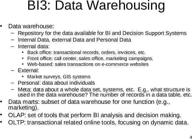
BI3: Data Warehousing Data warehouse: – Repository for the data available for BI and Decision Support Systems – Internal Data, external Data and Personal Data – Internal data: Back office: transactional records, orders, invoices, etc. Front office: call center, sales office, marketing campaigns, Web-based: sales transactions on e-commerce websites – External: Market surveys, GIS systems – Personal: data about individuals – Meta: data about a whole data set, systems, etc. E.g., what structure is used in the data warehouse? The number of records in a data table, etc. Data marts: subset of data warehouse for one function (e.g., marketing). OLAP: set of tools that perform BI analysis and decision making. OLTP: transactional related online tools, focusing on dynamic data. 4
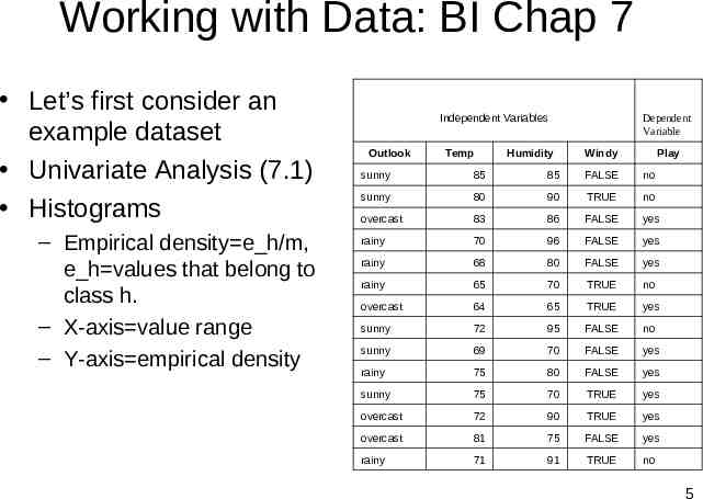
Working with Data: BI Chap 7 Let’s first consider an example dataset Univariate Analysis (7.1) Histograms – Empirical density e h/m, e h values that belong to class h. – X-axis value range – Y-axis empirical density Independent Variables Outlook Temp Humidity Dependent Variable Windy Play sunny 85 85 FALSE no sunny 80 90 TRUE no overcast 83 86 FALSE yes rainy 70 96 FALSE yes rainy 68 80 FALSE yes rainy 65 70 TRUE no overcast 64 65 TRUE yes sunny 72 95 FALSE no sunny 69 70 FALSE yes rainy 75 80 FALSE yes sunny 75 70 TRUE yes overcast 72 90 TRUE yes overcast 81 75 FALSE yes rainy 71 91 TRUE no 5
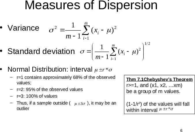
Measures of Dispersion Variance m 1 2 2 ( x ) i m 1 i 1 m 1 2 Standard deviation ( xi ) m 1 i 1 1/ 2 Normal Distribution: interval r * – r 1 contains approximately 68% of the observed values; – r 2: 95% of the observed values – r 3: 100% of values – Thus, if a sample outside ( 3 ), it may be an outlier Thm 7.1Chebyshev’s Theorem r 1, and (x1, x2, xm) be a group of m values. (1-1/r2) of the values will fall within interval r * 6
Heterogeneity Measures The Gini index (Wiki: The Gini coefficient (also known as the Gini index or Gini ratio) is a measure of statistical dispersion developed by the Italian statistician and sociologist Corrado Gini and published in his 1912 paper "Variability and Mutability" (Italian: Variabilità e mutabilità) ) Let fh be the frequency of class h; then G is Gini index Entropy E: 0 means lowest heterogeneity, and 1 highest. G 1 H f 2 h i 1 H E f h log 2 f h i1 7
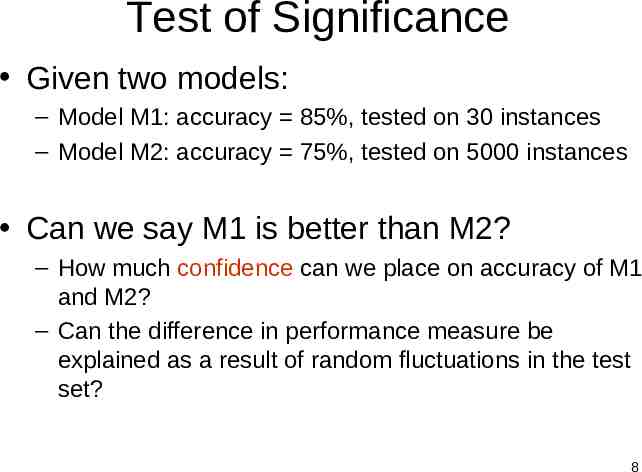
Test of Significance Given two models: – Model M1: accuracy 85%, tested on 30 instances – Model M2: accuracy 75%, tested on 5000 instances Can we say M1 is better than M2? – How much confidence can we place on accuracy of M1 and M2? – Can the difference in performance measure be explained as a result of random fluctuations in the test set? 8
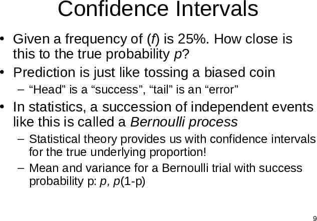
Confidence Intervals Given a frequency of (f) is 25%. How close is this to the true probability p? Prediction is just like tossing a biased coin – “Head” is a “success”, “tail” is an “error” In statistics, a succession of independent events like this is called a Bernoulli process – Statistical theory provides us with confidence intervals for the true underlying proportion! – Mean and variance for a Bernoulli trial with success probability p: p, p(1-p) 9
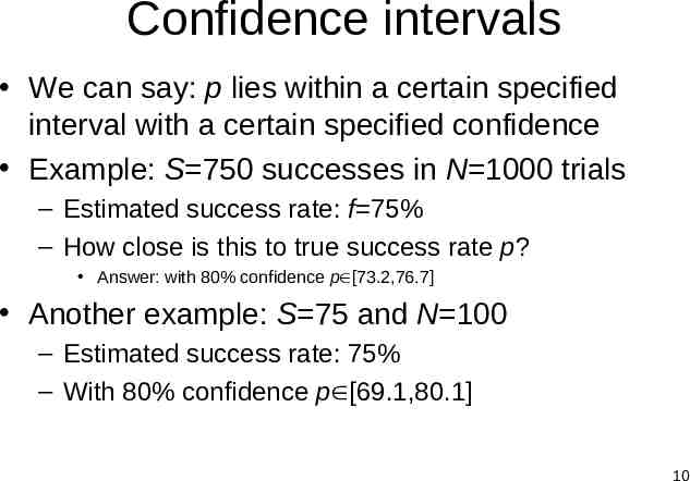
Confidence intervals We can say: p lies within a certain specified interval with a certain specified confidence Example: S 750 successes in N 1000 trials – Estimated success rate: f 75% – How close is this to true success rate p? Answer: with 80% confidence p [73.2,76.7] Another example: S 75 and N 100 – Estimated success rate: 75% – With 80% confidence p [69.1,80.1] 10
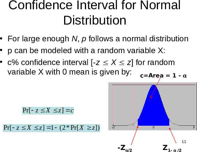
Confidence Interval for Normal Distribution For large enough N, p follows a normal distribution p can be modeled with a random variable X: c% confidence interval [-z X z] for random variable X with 0 mean is given by: c Area 1 - Pr[ z X z ] c Pr[ z X z ] 1 (2 * Pr[ X z ]) -Z /2 Z1- /2 11
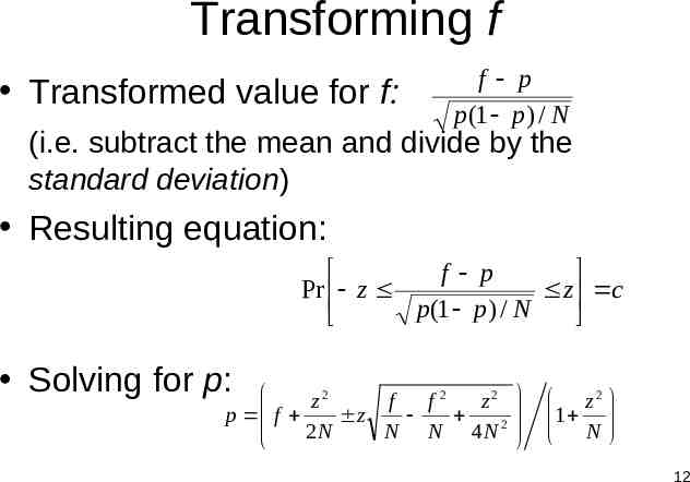
Transforming f Transformed value for f: f p p (1 p ) / N (i.e. subtract the mean and divide by the standard deviation) Resulting equation: f p Pr z z c p(1 p ) / N Solving for p: 2 2 2 z f f z p f z 2 2 N N N 4 N z2 1 N 12
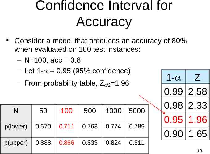
Confidence Interval for Accuracy Consider a model that produces an accuracy of 80% when evaluated on 100 test instances: – N 100, acc 0.8 – Let 1- 0.95 (95% confidence) – From probability table, Z /2 1.96 N 50 100 500 1000 5000 p(lower) 0.670 0.711 0.763 0.774 0.789 p(upper) 0.888 0.866 0.833 0.824 0.811 1- 0.99 0.98 0.95 0.90 Z 2.58 2.33 1.96 1.65 13
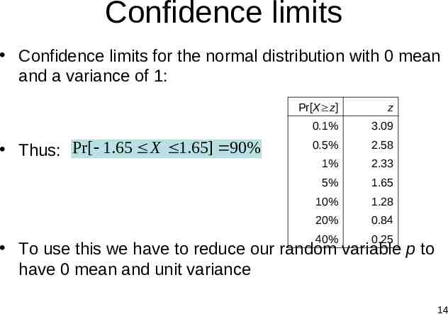
Confidence limits Confidence limits for the normal distribution with 0 mean and a variance of 1: Thus: Pr[ 1.65 X 1.65] 90% Pr[X z] z 0.1% 3.09 0.5% 2.58 1% 2.33 5% 1.65 10% 1.28 20% 0.84 40% 0.25 To use this we have to reduce our random variable p to have 0 mean and unit variance 14
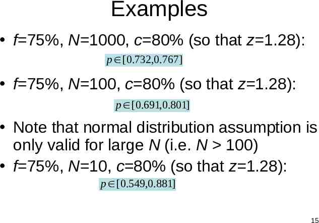
Examples f 75%, N 1000, c 80% (so that z 1.28): p [0.732,0.767] f 75%, N 100, c 80% (so that z 1.28): p [0.691,0.801] Note that normal distribution assumption is only valid for large N (i.e. N 100) f 75%, N 10, c 80% (so that z 1.28): p [0.549,0.881] 15
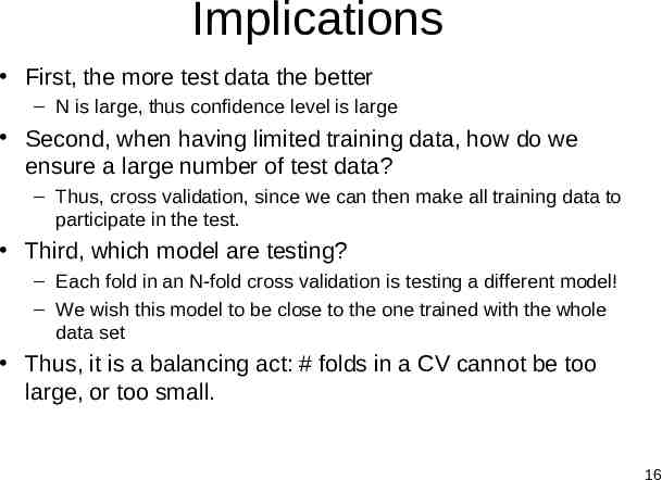
Implications First, the more test data the better – N is large, thus confidence level is large Second, when having limited training data, how do we ensure a large number of test data? – Thus, cross validation, since we can then make all training data to participate in the test. Third, which model are testing? – Each fold in an N-fold cross validation is testing a different model! – We wish this model to be close to the one trained with the whole data set Thus, it is a balancing act: # folds in a CV cannot be too large, or too small. 16
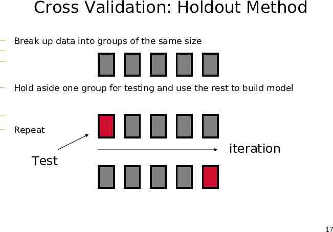
Cross Validation: Holdout Method — Break up data into groups of the same size — — — Hold aside one group for testing and use the rest to build model — — Repeat Test iteration 17
Cross Validation (CV) Natural performance measure for classification problems: error rate – #Success: instance’s class is predicted correctly – #Error: instance’s class is predicted incorrectly – Error rate: proportion of errors made over the whole set of instances Training Error vs. Test Error Confusion Matrix Confidence – 2% error in 100 tests – 2% error in 10000 tests Which one do you trust more? – Apply the confidence interval idea Tradeoff: – # of Folds # of Data N Leave One Out CV Trained model very close to final model, but test data very biased – # of Folds 2 Trained Model very unlike final model, but test data close to training distribution 18
ROC (Receiver Operating Characteristic) Page 298 of TSK book. Many applications care about ranking (give a queue from the most likely to the least likely) Examples Which ranking order is better? ROC: Developed in 1950s for signal detection theory to analyze noisy signals – Characterize the trade-off between positive hits and false alarms ROC curve plots TP (on the y-axis) against FP (on the x-axis) Performance of each classifier represented as a point on the ROC curve – changing the threshold of algorithm, sample distribution or cost matrix changes the location of the point 19
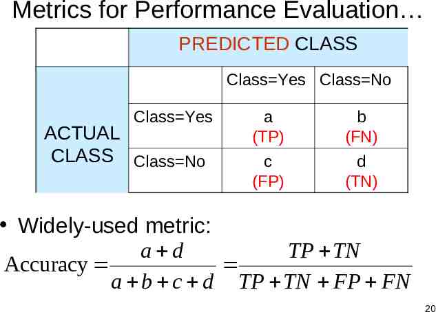
Metrics for Performance Evaluation PREDICTED CLASS Class Yes Class No Class Yes ACTUAL CLASS Class No a (TP) b (FN) c (FP) d (TN) Widely-used metric: a d TP TN Accuracy a b c d TP TN FP FN 20
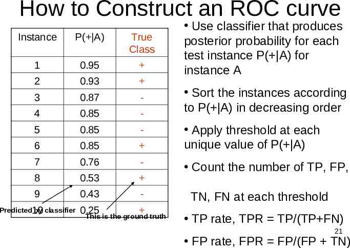
How to Construct an ROC curve Instance P( A) True Class 1 0.95 2 0.93 3 0.87 - 4 0.85 - 5 0.85 - 6 0.85 7 0.76 - 8 0.53 9 0.43 - Predicted10 by classifier 0.25 This is the ground truth Use classifier that produces posterior probability for each test instance P( A) for instance A Sort the instances according to P( A) in decreasing order Apply threshold at each unique value of P( A) Count the number of TP, FP, TN, FN at each threshold TP rate, TPR TP/(TP FN) 21 FP rate, FPR FP/(FP TN)
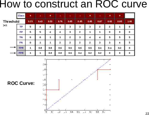
How to construct an ROC curve - - - - - 0.25 0.43 0.53 0.76 0.85 0.85 0.85 0.87 0.93 0.95 1.00 5 4 4 3 3 3 3 2 2 1 0 FP 5 5 4 4 3 2 1 1 0 0 0 TN 0 0 1 1 2 3 4 4 5 5 5 FN 0 1 1 2 2 2 2 3 3 4 5 TPR 1 0.8 0.8 0.6 0.6 0.6 0.6 0.4 0.4 0.2 0 FPR 1 1 0.8 0.8 0.6 0.4 0.2 0.2 0 0 0 Class P Threshold TP ROC Curve: 22
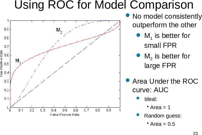
Using ROC for Model Comparison No model consistently outperform the other M is better for 1 small FPR M is better for 2 large FPR Area Under the ROC curve: AUC Ideal: Area 1 Random guess: Area 0.5 23
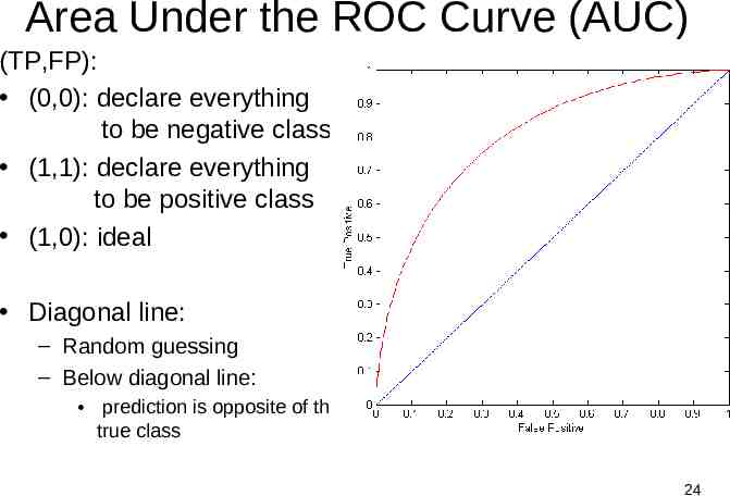
Area Under the ROC Curve (AUC) (TP,FP): (0,0): declare everything to be negative class (1,1): declare everything to be positive class (1,0): ideal Diagonal line: – Random guessing – Below diagonal line: prediction is opposite of the true class 24