CS 404/504 Special Topics: Adversarial Machine Learning Dr.
99 Slides8.77 MB
CS 404/504 Special Topics: Adversarial Machine Learning Dr. Alex Vakanski
CS 404/504, Fall 2021 Lecture 2 Deep Learning Overview 2
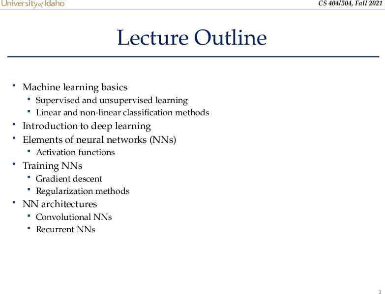
CS 404/504, Fall 2021 Lecture Outline Machine learning basics Supervised and unsupervised learning Linear and non-linear classification methods Introduction to deep learning Elements of neural networks (NNs) Activation functions Training NNs Gradient descent Regularization methods NN architectures Convolutional NNs Recurrent NNs 3
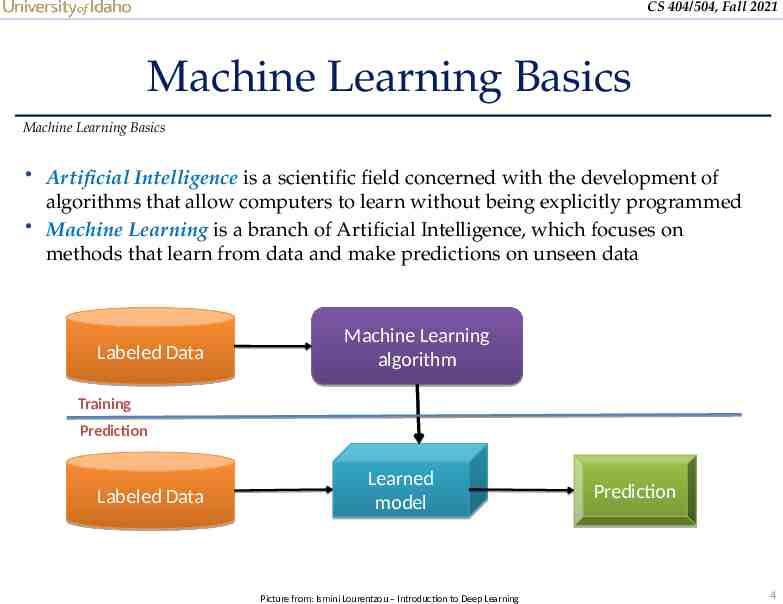
CS 404/504, Fall 2021 Machine Learning Basics Machine Learning Basics Artificial Intelligence is a scientific field concerned with the development of algorithms that allow computers to learn without being explicitly programmed Machine Learning is a branch of Artificial Intelligence, which focuses on methods that learn from data and make predictions on unseen data Labeled Data Machine Learning algorithm Training Prediction Labeled Data Learned model Picture from: Ismini Lourentzou – Introduction to Deep Learning Prediction 4
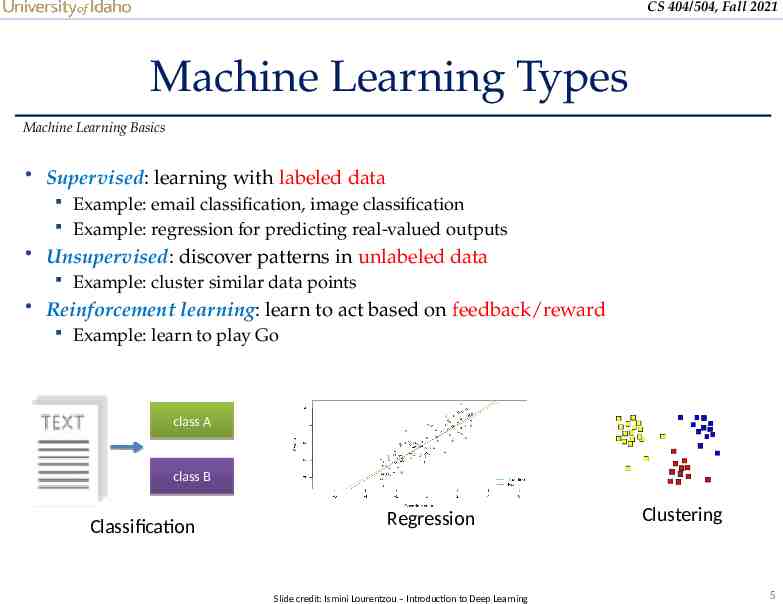
CS 404/504, Fall 2021 Machine Learning Types Machine Learning Basics Supervised: learning with labeled data Example: email classification, image classification Example: regression for predicting real-valued outputs Unsupervised: discover patterns in unlabeled data Example: cluster similar data points Reinforcement learning: learn to act based on feedback/reward Example: learn to play Go class A class B Classification Regression Slide credit: Ismini Lourentzou – Introduction to Deep Learning Clustering 5
CS 404/504, Fall 2021 Supervised Learning Machine Learning Basics Supervised learning categories and techniques Numerical classifier functions o Linear classifier, perceptron, logistic regression, support vector machines (SVM), neural networks Parametric (probabilistic) functions o Naïve Bayes, Gaussian discriminant analysis (GDA), hidden Markov models (HMM), probabilistic graphical models Non-parametric (instance-based) functions o k-nearest neighbors, kernel regression, kernel density estimation, local regression Symbolic functions o Decision trees, classification and regression trees (CART) Aggregation (ensemble) learning o Bagging, boosting (Adaboost), random forest Slide credit: Y-Fan Chang – An Overview of Machine Learning 6
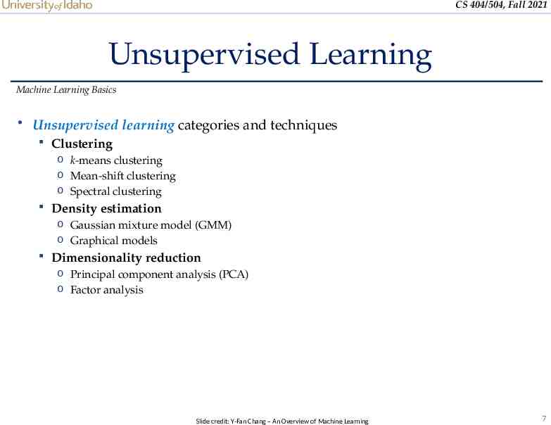
CS 404/504, Fall 2021 Unsupervised Learning Machine Learning Basics Unsupervised learning categories and techniques Clustering o k-means clustering o Mean-shift clustering o Spectral clustering Density estimation o Gaussian mixture model (GMM) o Graphical models Dimensionality reduction o Principal component analysis (PCA) o Factor analysis Slide credit: Y-Fan Chang – An Overview of Machine Learning 7
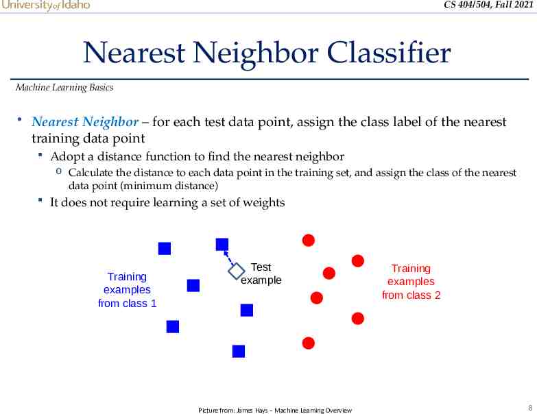
CS 404/504, Fall 2021 Nearest Neighbor Classifier Machine Learning Basics Nearest Neighbor – for each test data point, assign the class label of the nearest training data point Adopt a distance function to find the nearest neighbor o Calculate the distance to each data point in the training set, and assign the class of the nearest data point (minimum distance) It does not require learning a set of weights Training examples from class 1 Test example Picture from: James Hays – Machine Learning Overview Training examples from class 2 8
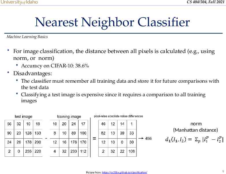
CS 404/504, Fall 2021 Nearest Neighbor Classifier Machine Learning Basics For image classification, the distance between all pixels is calculated (e.g., using norm, or norm) Accuracy on CIFAR-10: 38.6% Disadvantages: The classifier must remember all training data and store it for future comparisons with the test data Classifying a test image is expensive since it requires a comparison to all training images norm (Manhattan distance) Picture from: https://cs231n.github.io/classification/ 9
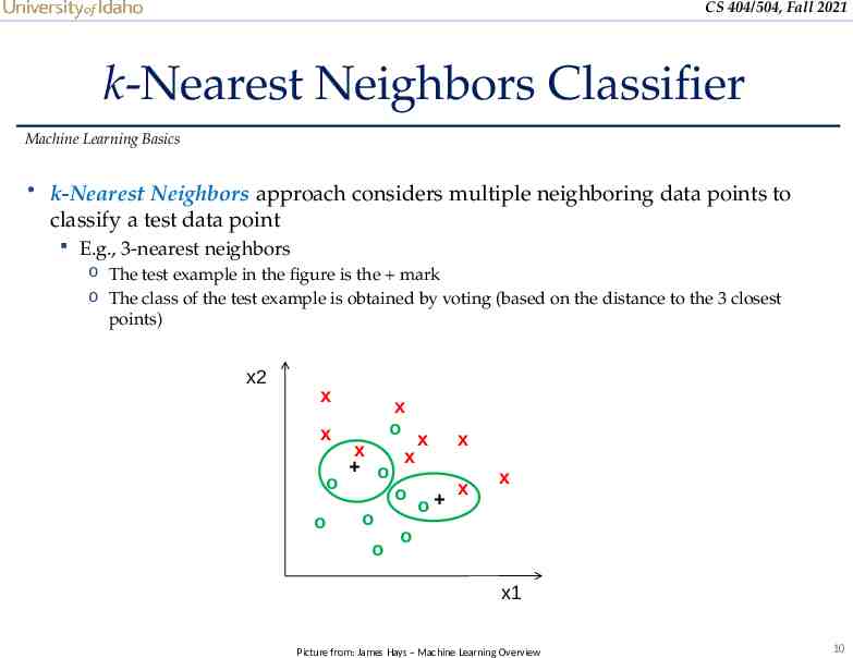
CS 404/504, Fall 2021 k-Nearest Neighbors Classifier Machine Learning Basics k-Nearest Neighbors approach considers multiple neighboring data points to classify a test data point E.g., 3-nearest neighbors o The test example in the figure is the mark o The class of the test example is obtained by voting (based on the distance to the 3 closest points) x2 x x o x x x x o x o o x o o o o o x x1 Picture from: James Hays – Machine Learning Overview 10
CS 404/504, Fall 2021 Linear Classifier Machine Learning Basics Linear classifier Find a linear function f of the inputs xi that separates the classes Use pairs of inputs and labels to find the weights matrix W and the bias vector b o The weights and biases are the parameters of the function f Several methods have been used to find the optimal set of parameters of a linear classifier o A common method of choice is the Perceptron algorithm, where the parameters are updated until a minimal error is reached (single layer, does not use backpropagation) Linear classifier is a simple approach, but it is a building block of advanced classification algorithms, such as SVM and neural networks o Earlier multi-layer neural networks were referred to as multi-layer perceptrons (MLPs) 11
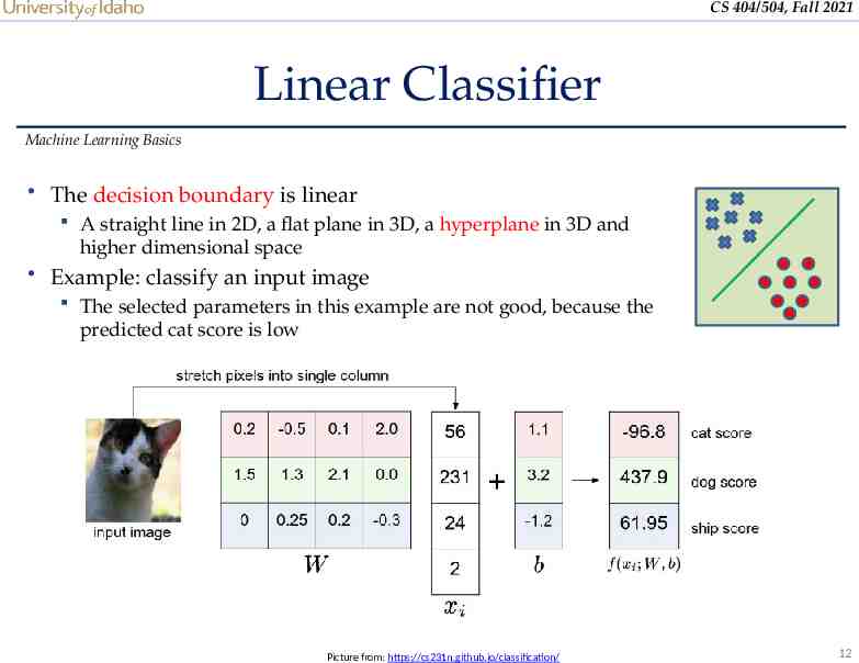
CS 404/504, Fall 2021 Linear Classifier Machine Learning Basics The decision boundary is linear A straight line in 2D, a flat plane in 3D, a hyperplane in 3D and higher dimensional space Example: classify an input image The selected parameters in this example are not good, because the predicted cat score is low Picture from: https://cs231n.github.io/classification/ 12
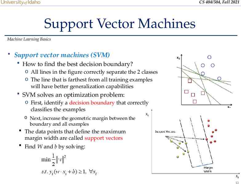
CS 404/504, Fall 2021 Support Vector Machines Machine Learning Basics Support vector machines (SVM) How to find the best decision boundary? o All lines in the figure correctly separate the 2 classes o The line that is farthest from all training examples will have better generalization capabilities SVM solves an optimization problem: o First, identify a decision boundary that correctly classifies the examples o Next, increase the geometric margin between the boundary and all examples The data points that define the maximum margin width are called support vectors Find W and b by solving: 13
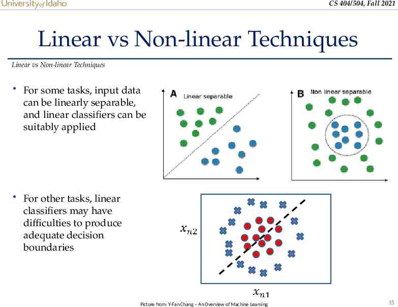
CS 404/504, Fall 2021 Linear vs Non-linear Techniques Linear vs Non-linear Techniques Linear classification techniques Linear classifier Perceptron Logistic regression Linear SVM Naïve Bayes Non-linear classification techniques k-nearest neighbors Non-linear SVM Neural networks Decision trees Random forest 14
CS 404/504, Fall 2021 Linear vs Non-linear Techniques Linear vs Non-linear Techniques For some tasks, input data can be linearly separable, and linear classifiers can be suitably applied For other tasks, linear classifiers may have difficulties to produce adequate decision boundaries Picture from: Y-Fan Chang – An Overview of Machine Learning 15
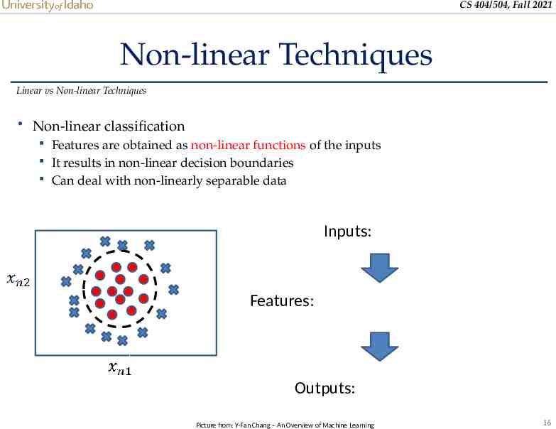
CS 404/504, Fall 2021 Non-linear Techniques Linear vs Non-linear Techniques Non-linear classification Features are obtained as non-linear functions of the inputs It results in non-linear decision boundaries Can deal with non-linearly separable data Inputs: Features: Outputs: Picture from: Y-Fan Chang – An Overview of Machine Learning 16
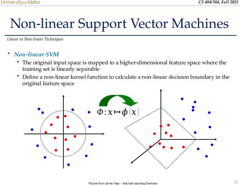
CS 404/504, Fall 2021 Non-linear Support Vector Machines Linear vs Non-linear Techniques Non-linear SVM The original input space is mapped to a higher-dimensional feature space where the training set is linearly separable Define a non-linear kernel function to calculate a non-linear decision boundary in the original feature space Φ : 𝑥 𝜙 (𝑥 ) Picture from: James Hays – Machine Learning Overview 17
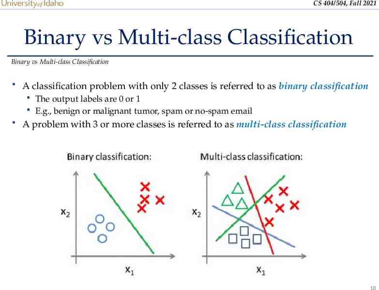
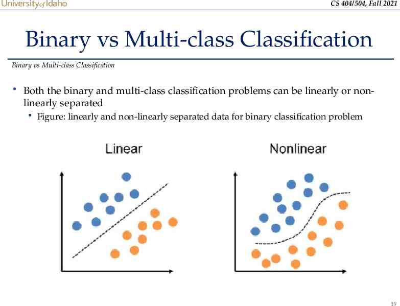
CS 404/504, Fall 2021 Binary vs Multi-class Classification Binary vs Multi-class Classification A classification problem with only 2 classes is referred to as binary classification The output labels are 0 or 1 E.g., benign or malignant tumor, spam or no-spam email A problem with 3 or more classes is referred to as multi-class classification 18
CS 404/504, Fall 2021 Binary vs Multi-class Classification Binary vs Multi-class Classification Both the binary and multi-class classification problems can be linearly or non- linearly separated Figure: linearly and non-linearly separated data for binary classification problem 19
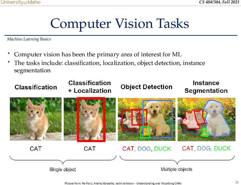
CS 404/504, Fall 2021 Computer Vision Tasks Machine Learning Basics Computer vision has been the primary area of interest for ML The tasks include: classification, localization, object detection, instance segmentation Picture from: Fie-Fei Li, Andrej Karpathy, Justin Johnson – Understanding and Visualizing CNNs 20
CS 404/504, Fall 2021 No-Free-Lunch Theorem Machine Learning Basics Wolpert (2002) - The Supervised Learning No-Free-Lunch Theorems The derived classification models for supervised learning are simplifications of the reality The simplifications are based on certain assumptions The assumptions fail in some situations o E.g., due to inability to perfectly estimate ML model parameters from limited data In summary, No-Free-Lunch Theorem states: No single classifier works the best for all possible problems Since we need to make assumptions to generalize 21
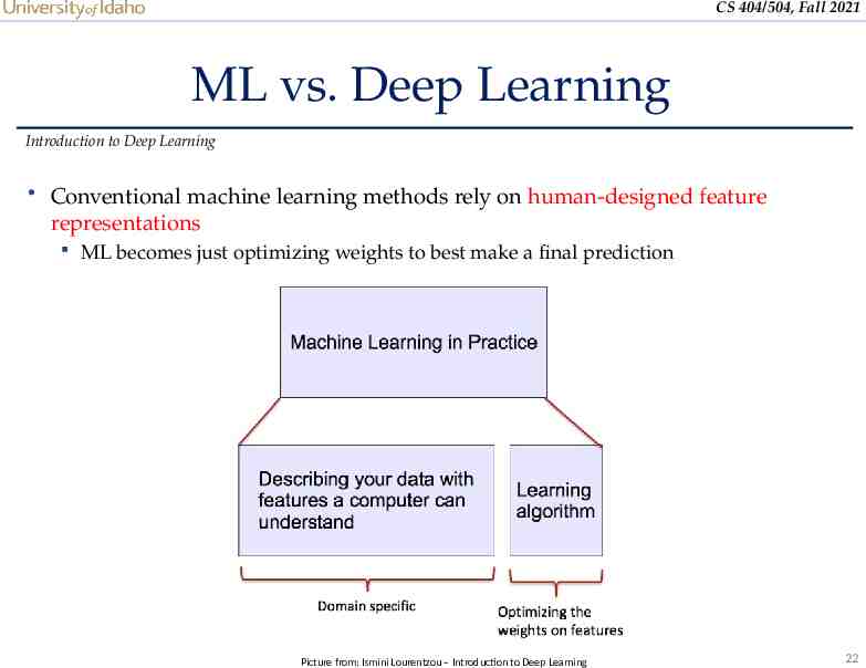
CS 404/504, Fall 2021 ML vs. Deep Learning Introduction to Deep Learning Conventional machine learning methods rely on human-designed feature representations ML becomes just optimizing weights to best make a final prediction Picture from: Ismini Lourentzou – Introduction to Deep Learning 22
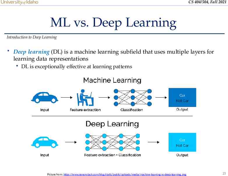
CS 404/504, Fall 2021 ML vs. Deep Learning Introduction to Deep Learning Deep learning (DL) is a machine learning subfield that uses multiple layers for learning data representations DL is exceptionally effective at learning patterns Picture from: https://www.xenonstack.com/blog/static/public/uploads/media/machine-learning-vs-deep-learning.png 23
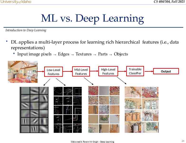
CS 404/504, Fall 2021 ML vs. Deep Learning Introduction to Deep Learning DL applies a multi-layer process for learning rich hierarchical features (i.e., data representations) Input image pixels Edges Textures Parts Objects Low-Level Features Mid-Level Features High-Level Features Slide credit: Param Vir Singh – Deep Learning Trainable Classifier Output 24
CS 404/504, Fall 2021 Why is DL Useful? Introduction to Deep Learning DL provides a flexible, learnable framework for representing visual, text, linguistic information Can learn in supervised and unsupervised manner DL represents an effective end-to-end learning system Requires large amounts of training data Since about 2010, DL has outperformed other ML techniques First in vision and speech, then NLP, and other applications 25
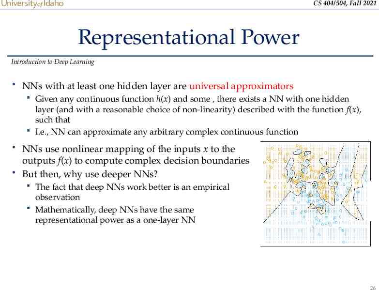
CS 404/504, Fall 2021 Representational Power Introduction to Deep Learning NNs with at least one hidden layer are universal approximators Given any continuous function h(x) and some , there exists a NN with one hidden layer (and with a reasonable choice of non-linearity) described with the function f(x), such that I.e., NN can approximate any arbitrary complex continuous function NNs use nonlinear mapping of the inputs x to the outputs f(x) to compute complex decision boundaries But then, why use deeper NNs? The fact that deep NNs work better is an empirical observation Mathematically, deep NNs have the same representational power as a one-layer NN 26
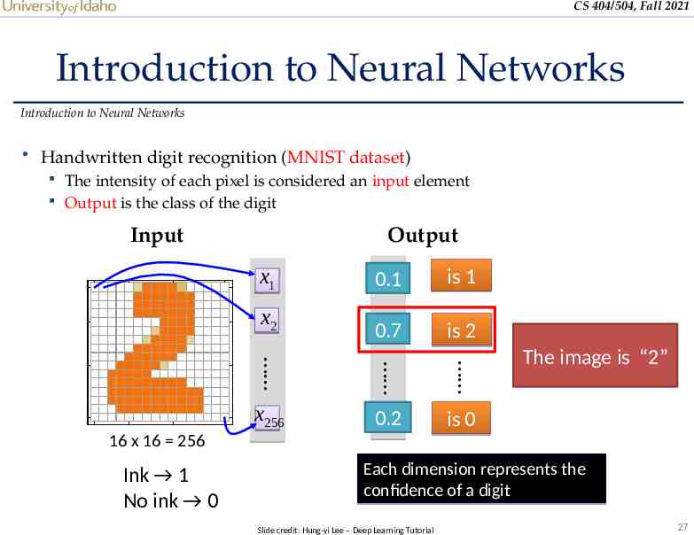
CS 404/504, Fall 2021 Introduction to Neural Networks Introduction to Neural Networks Handwritten digit recognition (MNIST dataset) The intensity of each pixel is considered an input element Output is the class of the digit Input Output x1 x2 0.7 y2 is 2 Ink 1 No ink 0 is 1 16 x 16 256 y1 0.1 x256 0.2 y10 is 0 The image is “2” Each dimension represents the confidence of a digit Slide credit: Hung-yi Lee – Deep Learning Tutorial 27
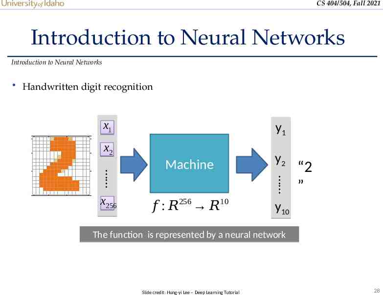
CS 404/504, Fall 2021 Introduction to Neural Networks Introduction to Neural Networks Handwritten digit recognition x1 y1 x2 y2 𝑓 : 𝑅256 𝑅10 y10 x256 Machine “2 ” The function is represented by a neural network Slide credit: Hung-yi Lee – Deep Learning Tutorial 28
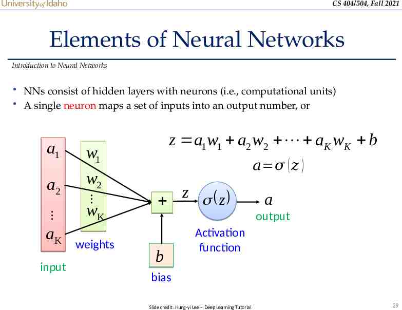
CS 404/504, Fall 2021 Elements of Neural Networks Introduction to Neural Networks NNs consist of hidden layers with neurons (i.e., computational units) A single neuron maps a set of inputs into an output number, or w1 a2 w2 wK aK input a1 weights z a1w1 a2 w2 aK wK b 𝑎 𝜎 ( 𝑧 ) z z a output b Activation function bias Slide credit: Hung-yi Lee – Deep Learning Tutorial 29
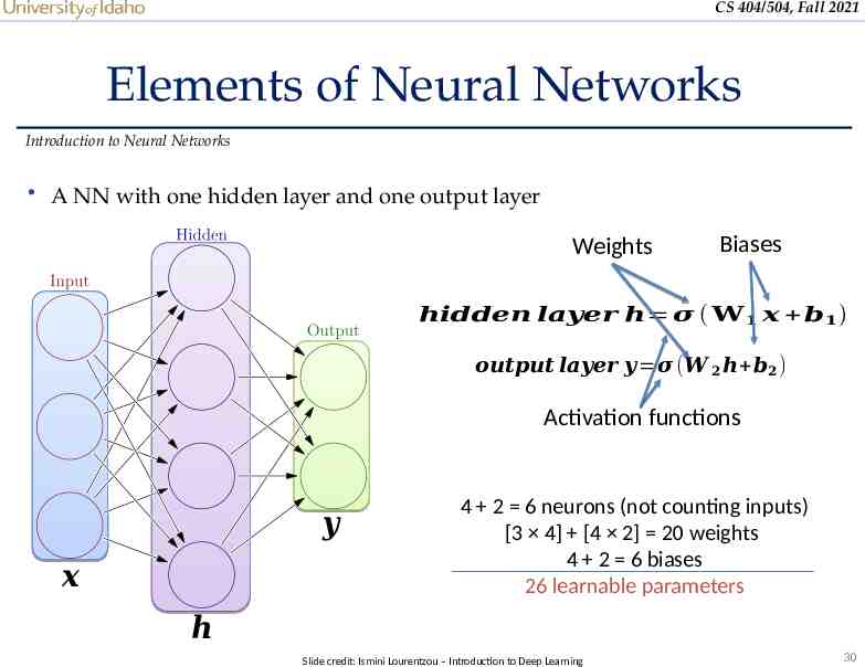
CS 404/504, Fall 2021 Elements of Neural Networks Introduction to Neural Networks A NN with one hidden layer and one output layer Weights Biases 𝒉𝒊𝒅𝒅𝒆𝒏 𝒍𝒂𝒚𝒆𝒓 𝒉 𝝈 ( 𝐖 𝟏 𝒙 𝒃𝟏 ) 𝒐𝒖𝒕𝒑𝒖𝒕 𝒍𝒂𝒚𝒆𝒓 𝒚 𝝈 (𝑾 𝟐 𝒉 𝒃𝟐 ) Activation functions 𝒚 𝒙 4 2 6 neurons (not counting inputs) [3 4] [4 2] 20 weights 4 2 6 biases 26 learnable parameters 𝒉 Slide credit: Ismini Lourentzou – Introduction to Deep Learning 30
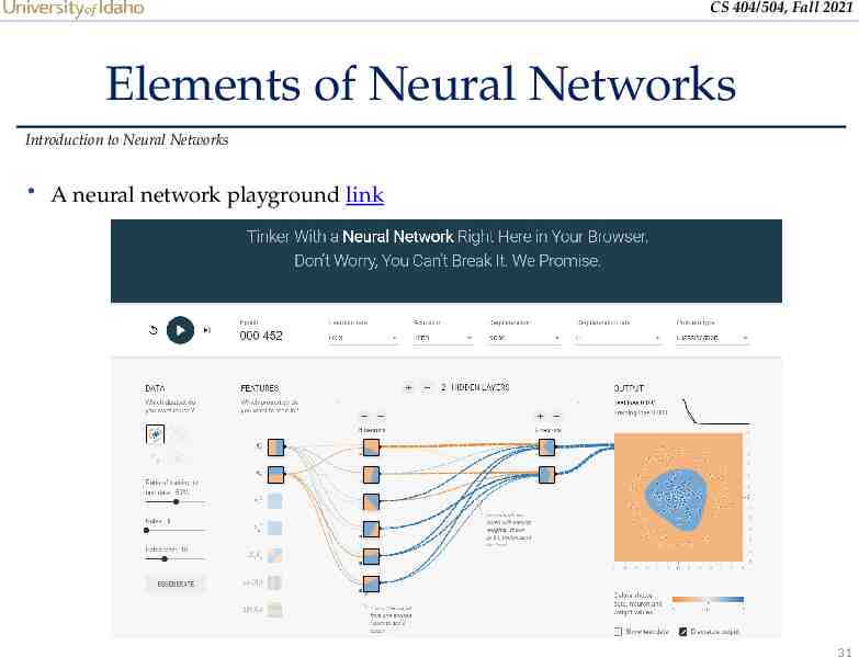
CS 404/504, Fall 2021 Elements of Neural Networks Introduction to Neural Networks A neural network playground link 31
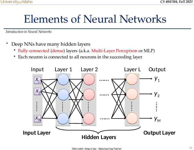
CS 404/504, Fall 2021 Elements of Neural Networks Introduction to Neural Networks Deep NNs have many hidden layers Fully-connected (dense) layers (a.k.a. Multi-Layer Perceptron or MLP) Each neuron is connected to all neurons in the succeeding layer Input Layer 1 Layer 2 Layer L Output x1 y1 x2 y2 Hidden Layers Slide credit: Hung-yi Lee – Deep Learning Tutorial Input Layer xN yM Output Layer 32
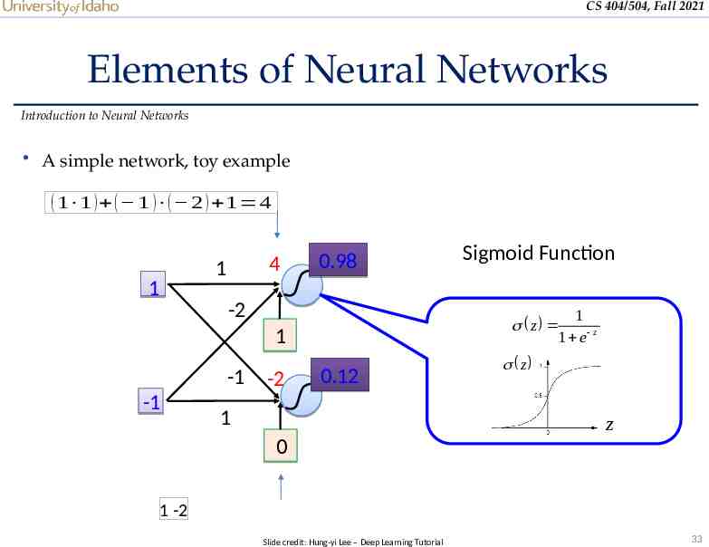
CS 404/504, Fall 2021 Elements of Neural Networks Introduction to Neural Networks A simple network, toy example ( 1 1 ) ( 1 ) ( 2 ) 1 4 4 1 1 0.98 -2 1 z 1 e z 1 -1 -1 -2 Sigmoid Function 0.12 1 z z 0 1 -2 Slide credit: Hung-yi Lee – Deep Learning Tutorial 33
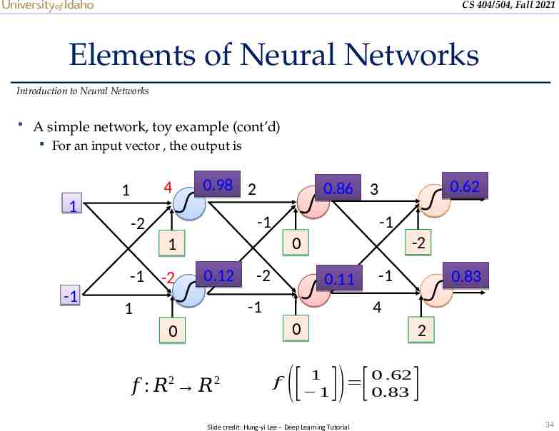
CS 404/504, Fall 2021 Elements of Neural Networks Introduction to Neural Networks A simple network, toy example (cont’d) For an input vector , the output is 1 4 1 0.98 2 -1 -2 -1 -1 -2 -2 0 1 -1 0.12 -2 0.11 -1 1 -1 0 𝑓 : 𝑅 𝑅 2 0.83 4 0 2 0.62 0.86 3 𝑓 2 1 1 ([ ]) [ Slide credit: Hung-yi Lee – Deep Learning Tutorial 0 .62 0.83 ] 34
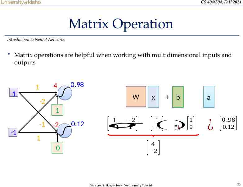
CS 404/504, Fall 2021 Matrix Operation Introduction to Neural Networks Matrix operations are helpful when working with multidimensional inputs and outputs 1 4 1 0.98 W -2 x b a 1 -1 -1 -2 1 0 0.12 1 2 𝜎 1 1 [ 1 ( 1 1 )0 0 .98 0.12 ] [ ] ¿ [ ] ¿ [ ] 4 [ 2 ] Slide credit: Hung-yi Lee – Deep Learning Tutorial 35
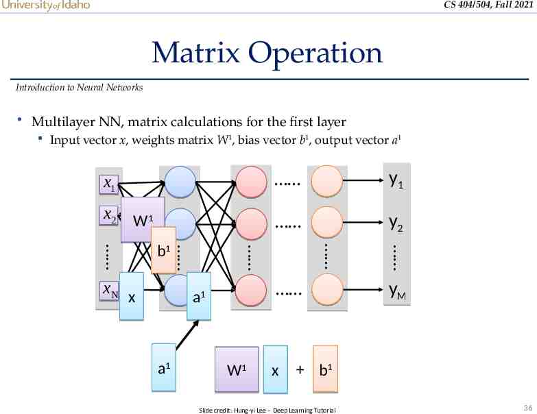
CS 404/504, Fall 2021 Matrix Operation Introduction to Neural Networks Multilayer NN, matrix calculations for the first layer Input vector x, weights matrix W1, bias vector b1, output vector a1 x1 y1 x 2 W1 y2 W1 x a1 a1 x xN b1 yM b1 Slide credit: Hung-yi Lee – Deep Learning Tutorial 36
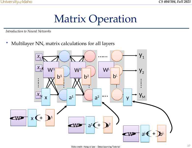
CS 404/504, Fall 2021 Matrix Operation Introduction to Neural Networks Multilayer NN, matrix calculations for all layers x1 x 2 W1 y2 a2 a1 bL 𝜎 b1 W1 x( ) WL b2 x y1 b1 xN W2 y yM 𝜎 b2 W2 a1( ) L-1 )L 𝜎 b WL a( Slide credit: Hung-yi Lee – Deep Learning Tutorial 37
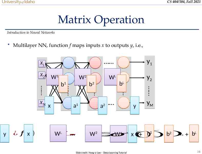
CS 404/504, Fall 2021 Matrix Operation Introduction to Neural Networks Multilayer NN, function f maps inputs x to outputs y, i.e., x1 x 2 W1 WL y2 ¿ WL a2 a1 bL ¿ 𝑓 ( x) y x y1 b2 b1 xN W2 y yM 𝜎 b1) W2 b2 bL 𝜎 W1 x( ( ) 𝜎 ( ) Slide credit: Hung-yi Lee – Deep Learning Tutorial 38
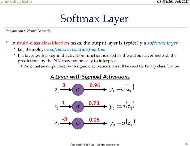
CS 404/504, Fall 2021 Softmax Layer Introduction to Neural Networks In multi-class classification tasks, the output layer is typically a softmax layer I.e., it employs a softmax activation function If a layer with a sigmoid activation function is used as the output layer instead, the predictions by the NN may not be easy to interpret o Note that an output layer with sigmoid activations can still be used for binary classification A Layer with Sigmoid Activations 3 0.95 z1 y1 z1 z2 1 z3 -3 0.73 y2 z 2 0.05 y3 z3 Slide credit: Hung-yi Lee – Deep Learning Tutorial 39
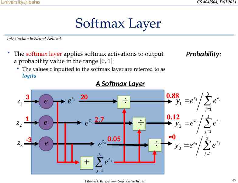
CS 404/504, Fall 2021 Softmax Layer Introduction to Neural Networks The softmax layer applies softmax activations to output Probability: a probability value in the range [0, 1] The values z inputted to the softmax layer are referred to as logits A Softmax Layer z1 3 e e z1 20 0.88 y1 e z1 3 e zj j 1 z2 1 z3 -3 e e e 2.7 z2 e z3 0.12 0.05 0 y3 e 3 e zj j 1 z3 3 e zj j 1 3 ez y2 e z2 j j 1 Slide credit: Hung-yi Lee – Deep Learning Tutorial 40
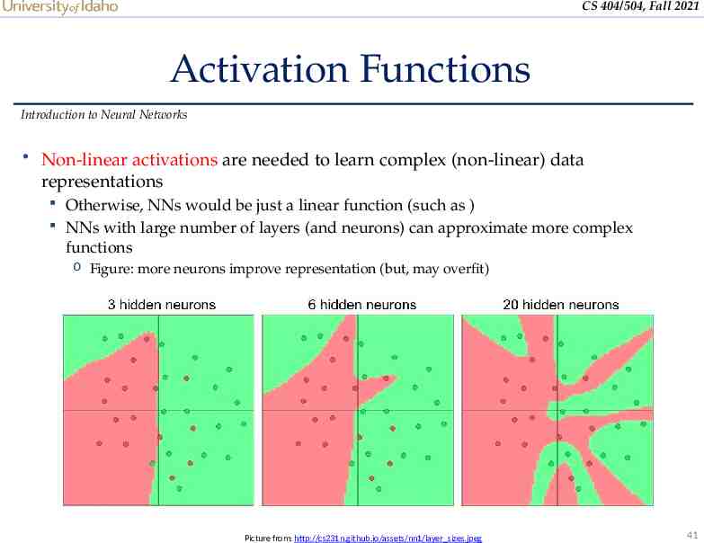
CS 404/504, Fall 2021 Activation Functions Introduction to Neural Networks Non-linear activations are needed to learn complex (non-linear) data representations Otherwise, NNs would be just a linear function (such as ) NNs with large number of layers (and neurons) can approximate more complex functions o Figure: more neurons improve representation (but, may overfit) Picture from: http://cs231n.github.io/assets/nn1/layer sizes.jpeg 41
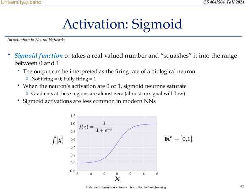
CS 404/504, Fall 2021 Activation: Sigmoid Introduction to Neural Networks Sigmoid function σ: takes a real-valued number and “squashes” it into the range between 0 and 1 The output can be interpreted as the firing rate of a biological neuron o Not firing 0; Fully firing 1 When the neuron’s activation are 0 or 1, sigmoid neurons saturate o Gradients at these regions are almost zero (almost no signal will flow) Sigmoid activations are less common in modern NNs ℝ 𝑛 [ 0,1 ] 𝑓 (𝑥 ) 𝑥 Slide credit: Ismini Lourentzou – Introduction to Deep Learning 42
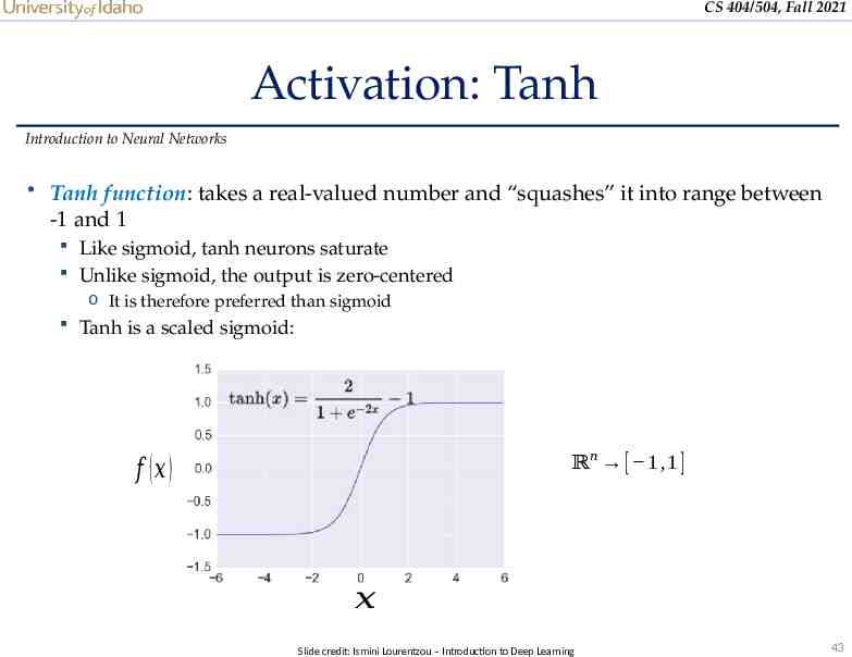
CS 404/504, Fall 2021 Activation: Tanh Introduction to Neural Networks Tanh function: takes a real-valued number and “squashes” it into range between -1 and 1 Like sigmoid, tanh neurons saturate Unlike sigmoid, the output is zero-centered o It is therefore preferred than sigmoid Tanh is a scaled sigmoid: ℝ 𝑛 [ 1 ,1 ] 𝑓 (𝑥 ) 𝑥 Slide credit: Ismini Lourentzou – Introduction to Deep Learning 43
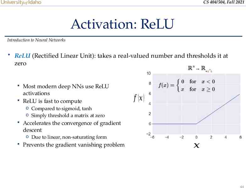
CS 404/504, Fall 2021 Activation: ReLU Introduction to Neural Networks ReLU (Rectified Linear Unit): takes a real-valued number and thresholds it at zero ℝ 𝑛 ℝ ¿ 𝑛 ¿ Most modern deep NNs use ReLU activations ReLU is fast to compute 𝑓 (𝑥 ) o Compared to sigmoid, tanh o Simply threshold a matrix at zero Accelerates the convergence of gradient descent o Due to linear, non-saturating form Prevents the gradient vanishing problem 𝑥 44
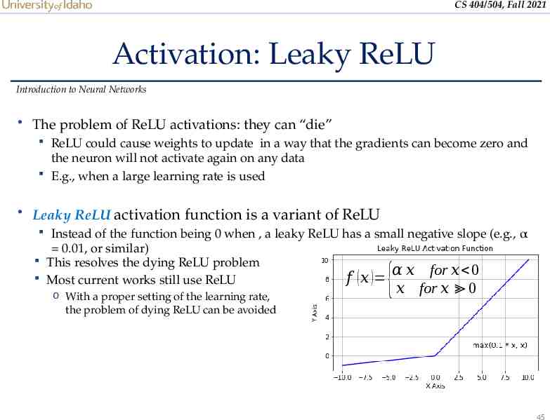
CS 404/504, Fall 2021 Activation: Leaky ReLU Introduction to Neural Networks The problem of ReLU activations: they can “die” ReLU could cause weights to update in a way that the gradients can become zero and the neuron will not activate again on any data E.g., when a large learning rate is used Leaky ReLU activation function is a variant of ReLU Instead of the function being 0 when , a leaky ReLU has a small negative slope (e.g., α 0.01, or similar) This resolves the dying ReLU problem 𝛼 𝑥 for 𝑥 0 Most current works still use ReLU 𝑓 ( 𝑥 ) o With a proper setting of the learning rate, the problem of dying ReLU can be avoided {𝑥 for 𝑥 0 45
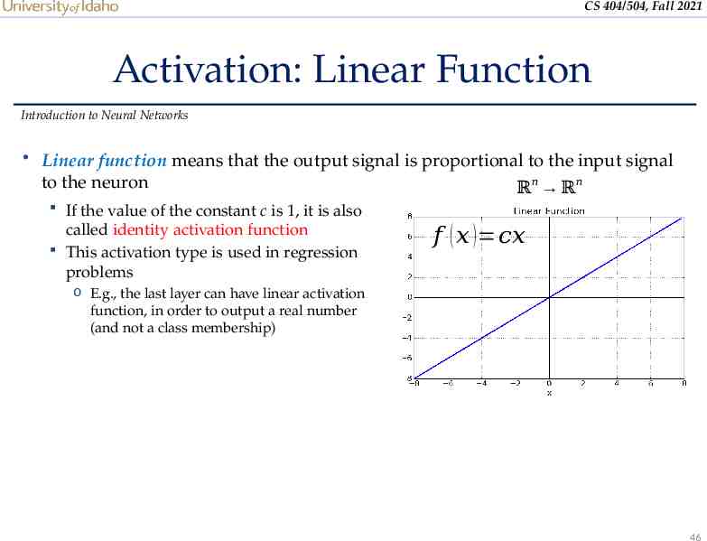
CS 404/504, Fall 2021 Activation: Linear Function Introduction to Neural Networks Linear function means that the output signal is proportional to the input signal to the neuron ℝ𝑛 ℝ𝑛 If the value of the constant c is 1, it is also called identity activation function This activation type is used in regression problems 𝑓 ( 𝑥 ) 𝑐𝑥 o E.g., the last layer can have linear activation function, in order to output a real number (and not a class membership) 46
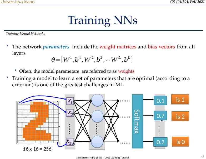
CS 404/504, Fall 2021 Training NNs Training Neural Networks The network parameters include the weight matrices and bias vectors from all layers 1 1 2 2 𝐿 𝐿 𝜃 { 𝑊 ,𝑏 , 𝑊 , 𝑏 , 𝑊 , 𝑏 } Often, the model parameters are referred to as weights Training a model to learn a set of parameters that are optimal (according to a criterion) is one of the greatest challenges in ML x2 16 x 16 256 Slide credit: Hung-yi Lee – Deep Learning Tutorial y1 0.1 is 1 0.7 y2 is 2 x256 Softmax x1 0.2 y10 is 0 47
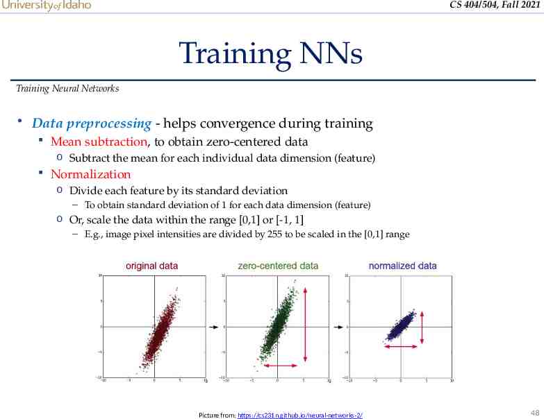
CS 404/504, Fall 2021 Training NNs Training Neural Networks Data preprocessing - helps convergence during training Mean subtraction, to obtain zero-centered data o Subtract the mean for each individual data dimension (feature) Normalization o Divide each feature by its standard deviation – To obtain standard deviation of 1 for each data dimension (feature) o Or, scale the data within the range [0,1] or [-1, 1] – E.g., image pixel intensities are divided by 255 to be scaled in the [0,1] range Picture from: https://cs231n.github.io/neural-networks-2/ 48
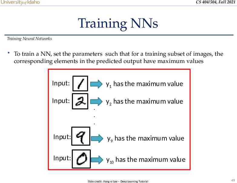
CS 404/504, Fall 2021 Training NNs Training Neural Networks To train a NN, set the parameters such that for a training subset of images, the corresponding elements in the predicted output have maximum values Input: y1 has the maximum value Input: y2 has the maximum value . . . Input: y9 has the maximum value Input: y10 has the maximum value Slide credit: Hung-yi Lee – Deep Learning Tutorial 49
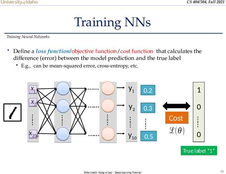
CS 404/504, Fall 2021 Training NNs Training Neural Networks Define a loss function/objective function/cost function that calculates the difference (error) between the model prediction and the true label E.g., can be mean-squared error, cross-entropy, etc. x1 y1 0.2 1 x2 y2 0.3 0 y10 0.5 x256 Cost ℒ(𝜃) 0 True label “1” Slide credit: Hung-yi Lee – Deep Learning Tutorial 50
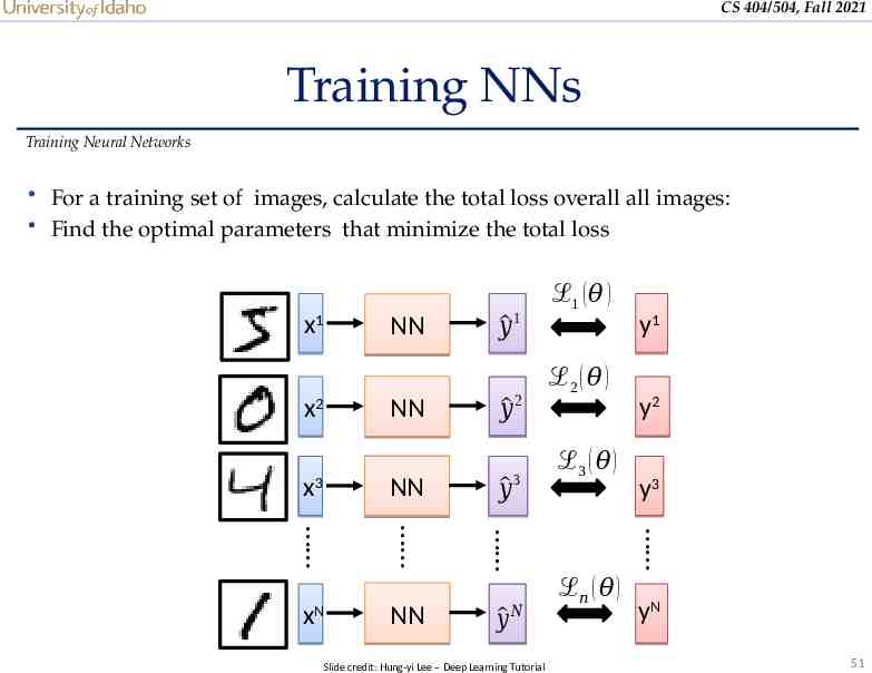
CS 404/504, Fall 2021 Training NNs Training Neural Networks For a training set of images, calculate the total loss overall all images: Find the optimal parameters that minimize the total loss x1 NN 𝑦 1 𝑦 2 x3 NN 𝑦 3 xN NN 𝑦 𝑁 Slide credit: Hung-yi Lee – Deep Learning Tutorial y1 ℒ2 ( 𝜃 ) ℒ3 ( 𝜃 ) y2 y3 NN x2 ℒ1 ( 𝜃 ) ℒ𝑛 ( 𝜃 ) yN 51
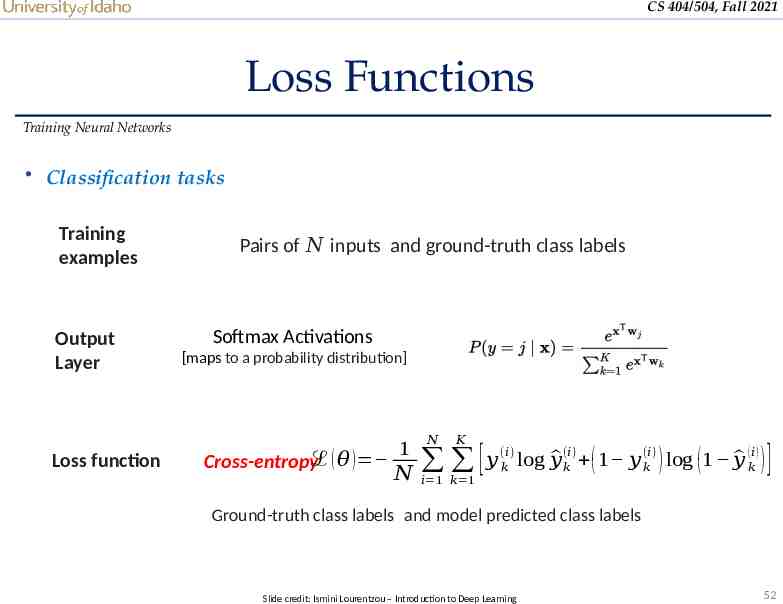
CS 404/504, Fall 2021 Loss Functions Training Neural Networks Classification tasks Training examples Output Layer Loss function Pairs of 𝑁 inputs and ground-truth class labels Softmax Activations [maps to a probability distribution] 1 Cross-entropyℒ ( 𝜃 ) 𝑁 𝑁 𝐾 [ 𝑦 (𝑖𝑘 ) log 𝑦 (𝑖𝑘 ) ( 1 𝑦 (𝑖𝑘 ) ) log (1 𝑦 (𝑘𝑖 ) ) ] 𝑖 1 𝑘 1 Ground-truth class labels and model predicted class labels Slide credit: Ismini Lourentzou – Introduction to Deep Learning 52
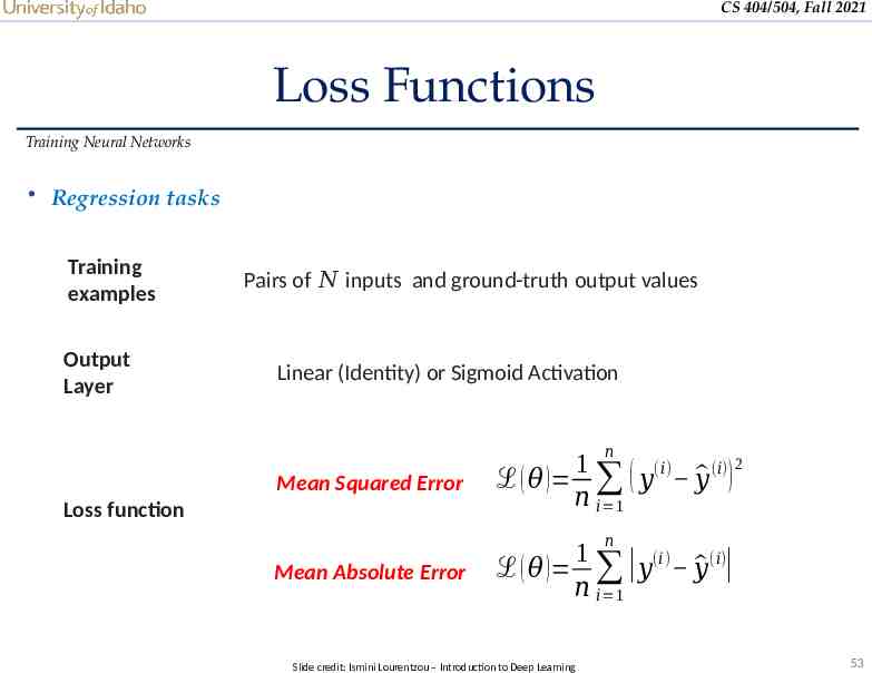
CS 404/504, Fall 2021 Loss Functions Training Neural Networks Regression tasks Training examples Output Layer Pairs of 𝑁 inputs and ground-truth output values Linear (Identity) or Sigmoid Activation 𝑛 Mean Squared Error Loss function 1 (𝑖) (𝑖) 2 ℒ ( 𝜃 ) ( 𝑦 𝑦 ) 𝑛 𝑖 1 𝑛 Mean Absolute Error ℒ ( 𝜃 ) 1 (𝑖) (𝑖) 𝑦 𝑦 𝑛 𝑖 1 Slide credit: Ismini Lourentzou – Introduction to Deep Learning 53
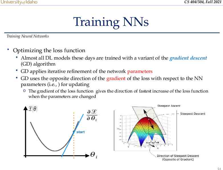
CS 404/504, Fall 2021 Training NNs Training Neural Networks Optimizing the loss function Almost all DL models these days are trained with a variant of the gradient descent (GD) algorithm GD applies iterative refinement of the network parameters GD uses the opposite direction of the gradient of the loss with respect to the NN parameters (i.e., ) for updating o The gradient of the loss function gives the direction of fastest increase of the loss function when the parameters are changed ℒ( 𝜃) ℒ 𝜃𝑖 𝜃𝑖 54
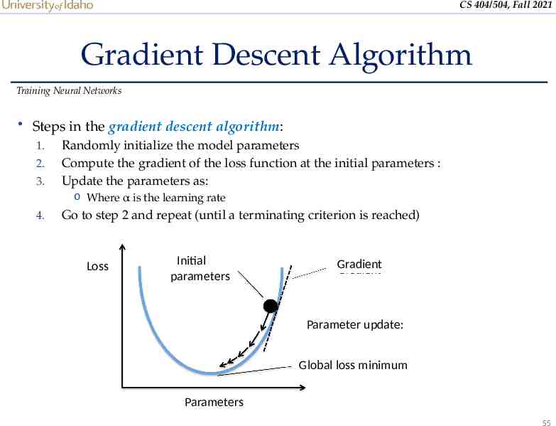
CS 404/504, Fall 2021 Gradient Descent Algorithm Training Neural Networks Steps in the gradient descent algorithm: 1. Randomly initialize the model parameters 2. Compute the gradient of the loss function at the initial parameters : 3. Update the parameters as: o Where α is the learning rate 4. Go to step 2 and repeat (until a terminating criterion is reached) Loss Initial parameters Gradient Parameter update: Global loss minimum Parameters 55
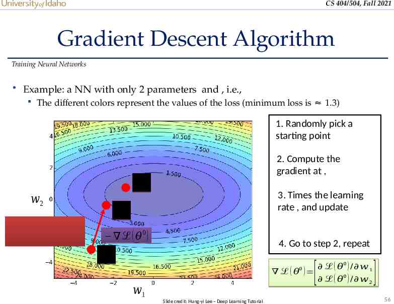
CS 404/504, Fall 2021 Gradient Descent Algorithm Training Neural Networks Example: a NN with only 2 parameters and , i.e., The different colors represent the values of the loss (minimum loss is 1.3) 1. Randomly pick a starting point 2. Compute the gradient at , 𝜃 𝑤2 𝜃 3. Times the learning rate , and update 1 ℒ ( 𝜃0 ) 𝜃 4. Go to step 2, repeat 0 ℒ ( 𝜃 0 ) / 𝑤 1 ℒ ( 𝜃 ) 0 ℒ ( 𝜃 ) / 𝑤 2 0 𝑤1 Slide credit: Hung-yi Lee – Deep Learning Tutorial [ ] 56
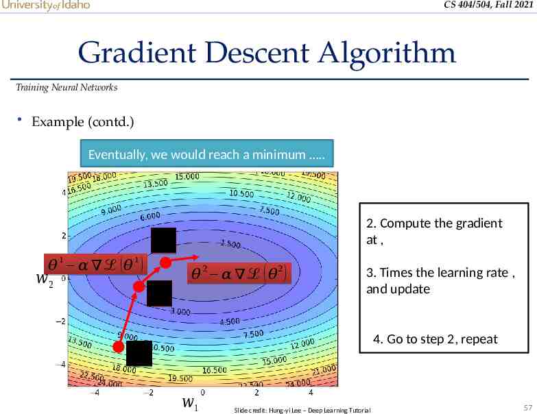
CS 404/504, Fall 2021 Gradient Descent Algorithm Training Neural Networks Example (contd.) Eventually, we would reach a minimum . 2. Compute the gradient at , 𝜃2 𝜃 1 𝛼 ℒ (𝜃 1) 𝑤2 𝜃1 𝜃 𝜃 2 𝛼 ℒ ( 𝜃2 ) 3. Times the learning rate , and update 4. Go to step 2, repeat 0 𝑤1 Slide credit: Hung-yi Lee – Deep Learning Tutorial 57
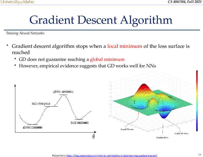
CS 404/504, Fall 2021 Gradient Descent Algorithm Training Neural Networks Gradient descent algorithm stops when a local minimum of the loss surface is reached GD does not guarantee reaching a global minimum However, empirical evidence suggests that GD works well for NNs 𝜃 Picture from: https://blog.paperspace.com/intro-to-optimization-in-deep-learning-gradient-descent/ 58
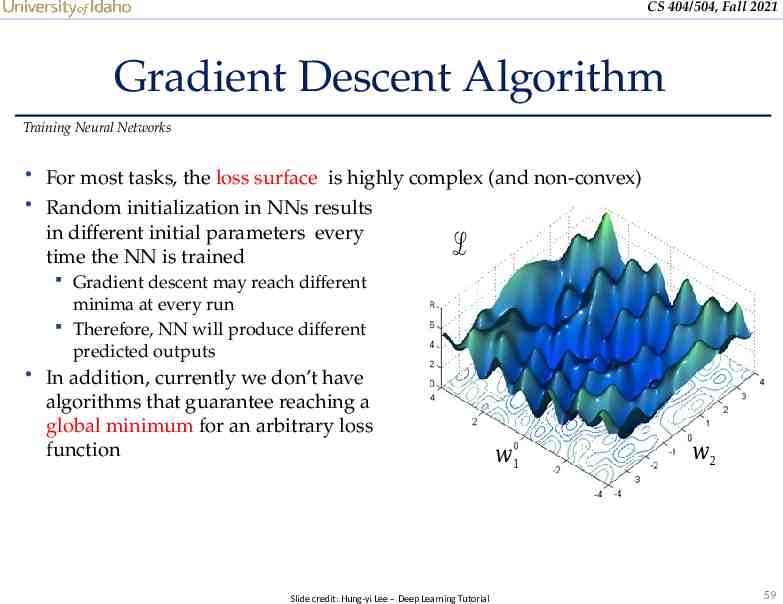
CS 404/504, Fall 2021 Gradient Descent Algorithm Training Neural Networks For most tasks, the loss surface is highly complex (and non-convex) Random initialization in NNs results in different initial parameters every time the NN is trained ℒ Gradient descent may reach different minima at every run Therefore, NN will produce different predicted outputs In addition, currently we don’t have algorithms that guarantee reaching a global minimum for an arbitrary loss function Slide credit: Hung-yi Lee – Deep Learning Tutorial 𝑤1 𝑤2 59
CS 404/504, Fall 2021 Backpropagation Training Neural Networks Modern NNs employ the backpropagation method for calculating the gradients of the loss function Backpropagation is short for “backward propagation” For training NNs, forward propagation (forward pass) refers to passing the inputs through the hidden layers to obtain the model outputs (predictions) The loss function is then calculated Backpropagation traverses the network in reverse order, from the outputs backward toward the inputs to calculate the gradients of the loss The chain rule is used for calculating the partial derivatives of the loss function with respect to the parameters in the different layers in the network Each update of the model parameters during training takes one forward and one backward pass (e.g., of a batch of inputs) Automatic calculation of the gradients (automatic differentiation) is available in all current deep learning libraries It significantly simplifies the implementation of deep learning algorithms, since it obviates deriving the partial derivatives of the loss function by hand 60
CS 404/504, Fall 2021 Mini-batch Gradient Descent Training Neural Networks It is wasteful to compute the loss over the entire training dataset to perform a single parameter update for large datasets E.g., ImageNet has 14M images Therefore, GD (a.k.a. vanilla GD) is almost always replaced with mini-batch GD Mini-batch gradient descent Approach: o Compute the loss on a mini-batch of images, update the parameters , and repeat until all images are used o At the next epoch, shuffle the training data, and repeat the above process Mini-batch GD results in much faster training Typical mini-batch size: 32 to 256 images It works because the gradient from a mini-batch is a good approximation of the gradient from the entire training set 61
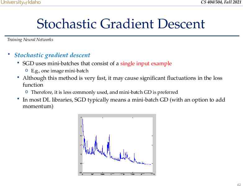
CS 404/504, Fall 2021 Stochastic Gradient Descent Training Neural Networks Stochastic gradient descent SGD uses mini-batches that consist of a single input example o E.g., one image mini-batch Although this method is very fast, it may cause significant fluctuations in the loss function o Therefore, it is less commonly used, and mini-batch GD is preferred In most DL libraries, SGD typically means a mini-batch GD (with an option to add momentum) 62
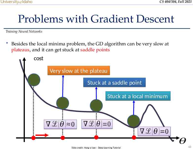
CS 404/504, Fall 2021 Problems with Gradient Descent Training Neural Networks Besides the local minima problem, the GD algorithm can be very slow at plateaus, and it can get stuck at saddle points cost Very slow at the plateau Stuck at a saddle point Stuck at a local minimum ℒ (𝜃 ) 0 ℒ ( 𝜃 ) 0 ℒ ( 𝜃 ) 0 𝜃 Slide credit: Hung-yi Lee – Deep Learning Tutorial 63
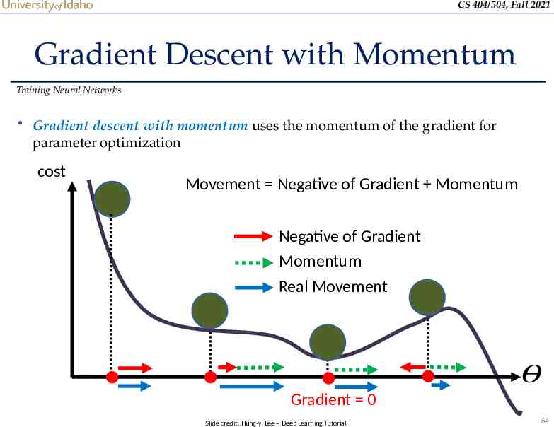
CS 404/504, Fall 2021 Gradient Descent with Momentum Training Neural Networks Gradient descent with momentum uses the momentum of the gradient for parameter optimization cost Movement Negative of Gradient Momentum Negative of Gradient Momentum Real Movement 𝜃 Gradient 0 Slide credit: Hung-yi Lee – Deep Learning Tutorial 64
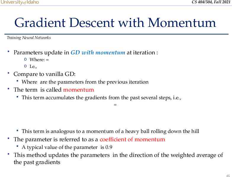
CS 404/504, Fall 2021 Gradient Descent with Momentum Training Neural Networks Parameters update in GD with momentum at iteration : o Where: o I.e., Compare to vanilla GD: Where are the parameters from the previous iteration The term is called momentum This term accumulates the gradients from the past several steps, i.e., This term is analogous to a momentum of a heavy ball rolling down the hill The parameter is referred to as a coefficient of momentum A typical value of the parameter is 0.9 This method updates the parameters in the direction of the weighted average of the past gradients 65
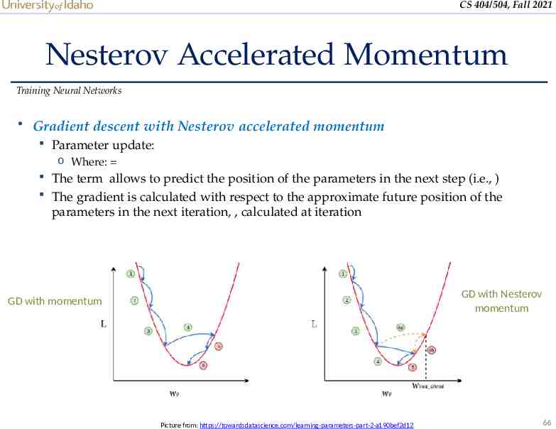
CS 404/504, Fall 2021 Nesterov Accelerated Momentum Training Neural Networks Gradient descent with Nesterov accelerated momentum Parameter update: o Where: The term allows to predict the position of the parameters in the next step (i.e., ) The gradient is calculated with respect to the approximate future position of the parameters in the next iteration, , calculated at iteration GD with Nesterov momentum GD with momentum Picture from: https://towardsdatascience.com/learning-parameters-part-2-a190bef2d12 66
CS 404/504, Fall 2021 Adam Training Neural Networks Adaptive Moment Estimation (Adam) Adam combines insights from the momentum optimizers that accumulate the values of past gradients, and it also introduces new terms based on the second moment of the gradient o Similar to GD with momentum, Adam computes a weighted average of past gradients (first moment of the gradient), i.e., o Adam also computes a weighted average of past squared gradients (second moment of the gradient), , i.e., The parameter update is: o Where: and o The proposed default values are 0.9, 0.999, and Other commonly used optimization methods include: Adagrad, Adadelta, RMSprop, Nadam, etc. Most commonly used optimizers nowadays are Adam and SGD with momentum 67
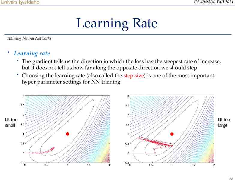
CS 404/504, Fall 2021 Learning Rate Training Neural Networks Learning rate The gradient tells us the direction in which the loss has the steepest rate of increase, but it does not tell us how far along the opposite direction we should step Choosing the learning rate (also called the step size) is one of the most important hyper-parameter settings for NN training LR too small LR too large 68
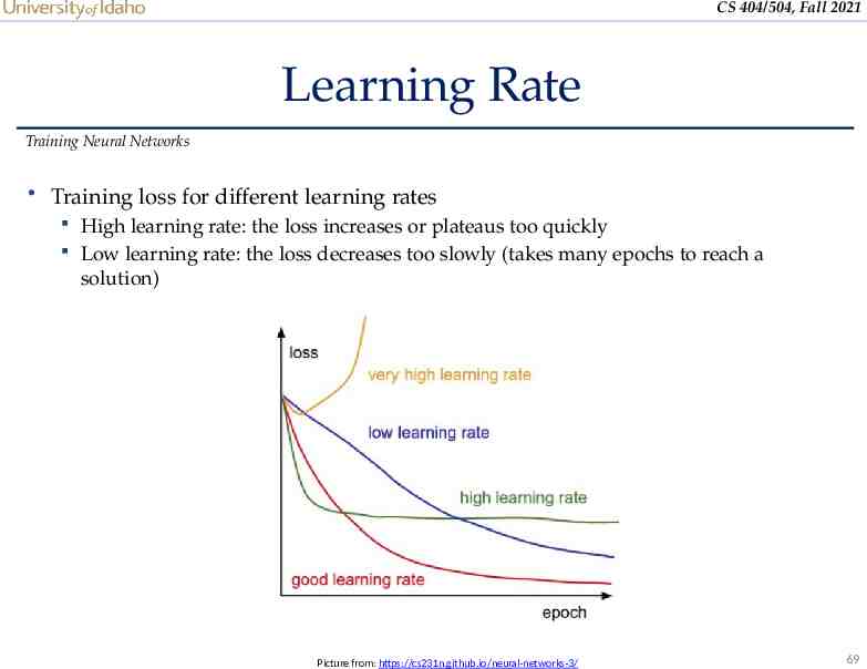
CS 404/504, Fall 2021 Learning Rate Training Neural Networks Training loss for different learning rates High learning rate: the loss increases or plateaus too quickly Low learning rate: the loss decreases too slowly (takes many epochs to reach a solution) Picture from: https://cs231n.github.io/neural-networks-3/ 69
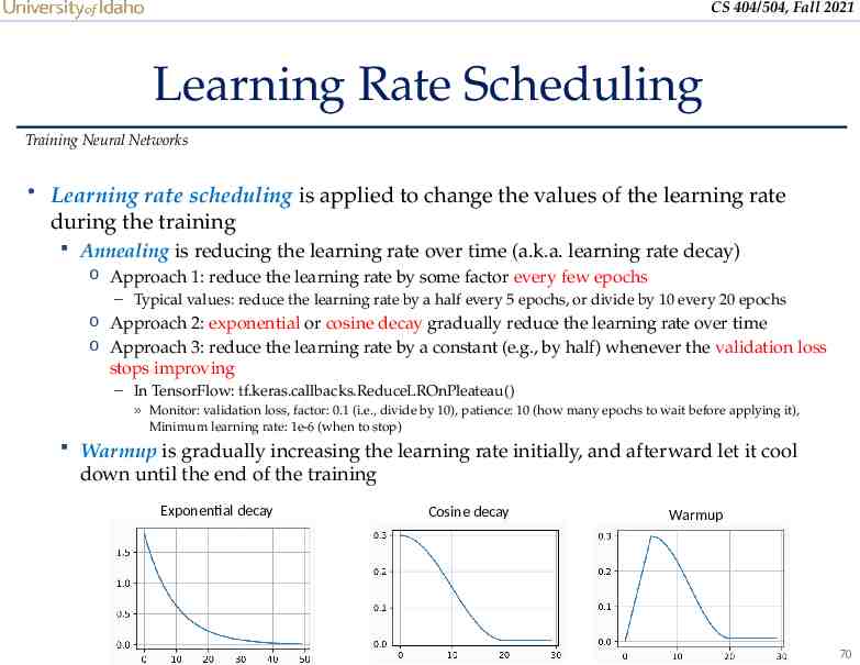
CS 404/504, Fall 2021 Learning Rate Scheduling Training Neural Networks Learning rate scheduling is applied to change the values of the learning rate during the training Annealing is reducing the learning rate over time (a.k.a. learning rate decay) o Approach 1: reduce the learning rate by some factor every few epochs – Typical values: reduce the learning rate by a half every 5 epochs, or divide by 10 every 20 epochs o Approach 2: exponential or cosine decay gradually reduce the learning rate over time o Approach 3: reduce the learning rate by a constant (e.g., by half) whenever the validation loss stops improving – In TensorFlow: tf.keras.callbacks.ReduceLROnPleateau() » Monitor: validation loss, factor: 0.1 (i.e., divide by 10), patience: 10 (how many epochs to wait before applying it), Minimum learning rate: 1e-6 (when to stop) Warmup is gradually increasing the learning rate initially, and afterward let it cool down until the end of the training Exponential decay Cosine decay Warmup 70
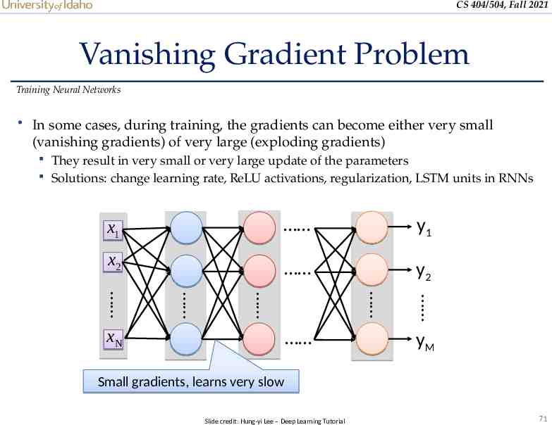
CS 404/504, Fall 2021 Vanishing Gradient Problem Training Neural Networks In some cases, during training, the gradients can become either very small (vanishing gradients) of very large (exploding gradients) They result in very small or very large update of the parameters Solutions: change learning rate, ReLU activations, regularization, LSTM units in RNNs x1 y1 x2 y2 xN yM Small gradients, learns very slow Slide credit: Hung-yi Lee – Deep Learning Tutorial 71
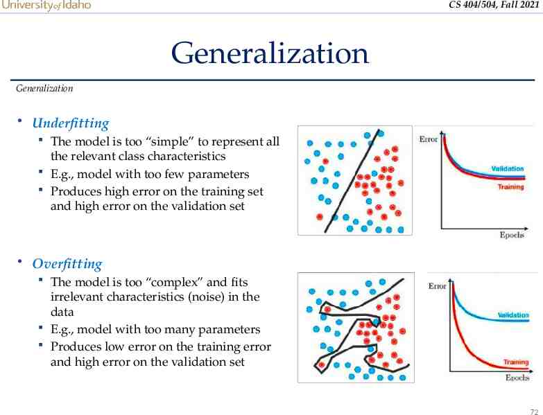
CS 404/504, Fall 2021 Generalization Generalization Underfitting The model is too “simple” to represent all the relevant class characteristics E.g., model with too few parameters Produces high error on the training set and high error on the validation set Overfitting The model is too “complex” and fits irrelevant characteristics (noise) in the data E.g., model with too many parameters Produces low error on the training error and high error on the validation set 72
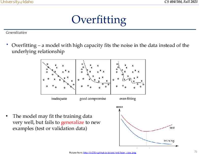
CS 404/504, Fall 2021 Overfitting Generalization Overfitting – a model with high capacity fits the noise in the data instead of the underlying relationship The model may fit the training data very well, but fails to generalize to new examples (test or validation data) Picture from: http://cs231n.github.io/assets/nn1/layer sizes.jpeg 73
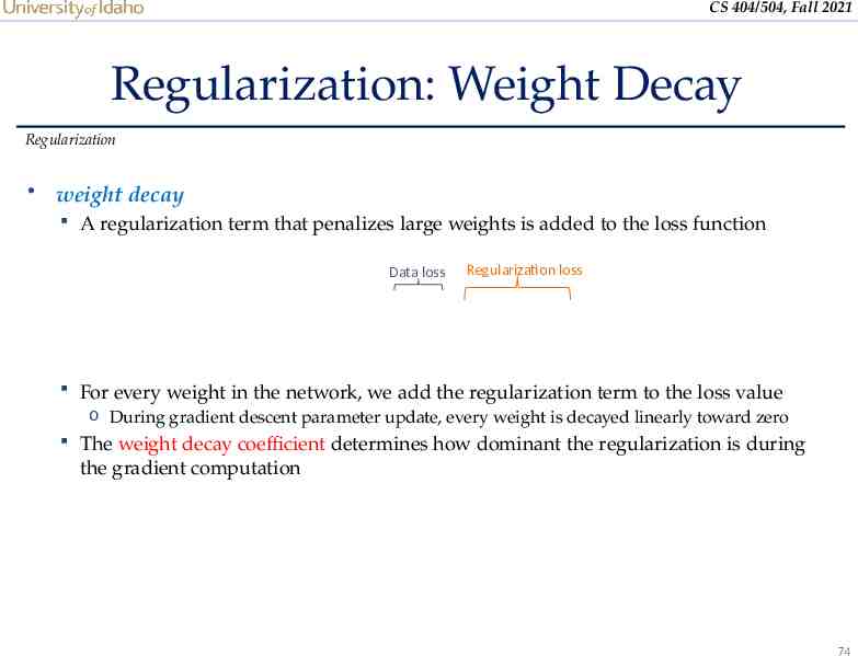
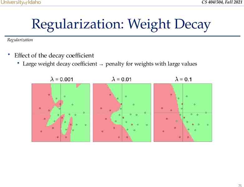
CS 404/504, Fall 2021 Regularization: Weight Decay Regularization weight decay A regularization term that penalizes large weights is added to the loss function Data loss Regularization loss For every weight in the network, we add the regularization term to the loss value o During gradient descent parameter update, every weight is decayed linearly toward zero The weight decay coefficient determines how dominant the regularization is during the gradient computation 74
CS 404/504, Fall 2021 Regularization: Weight Decay Regularization Effect of the decay coefficient Large weight decay coefficient penalty for weights with large values 75
CS 404/504, Fall 2021 Regularization: Weight Decay Regularization weight decay The regularization term is based on the norm of the weights weight decay is less common with NN o Often performs worse than weight decay It is also possible to combine and regularization o Called elastic net regularization 76
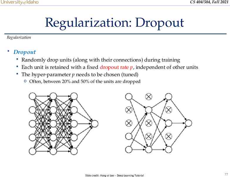
CS 404/504, Fall 2021 Regularization: Dropout Regularization Dropout Randomly drop units (along with their connections) during training Each unit is retained with a fixed dropout rate p, independent of other units The hyper-parameter p needs to be chosen (tuned) o Often, between 20% and 50% of the units are dropped Slide credit: Hung-yi Lee – Deep Learning Tutorial 77
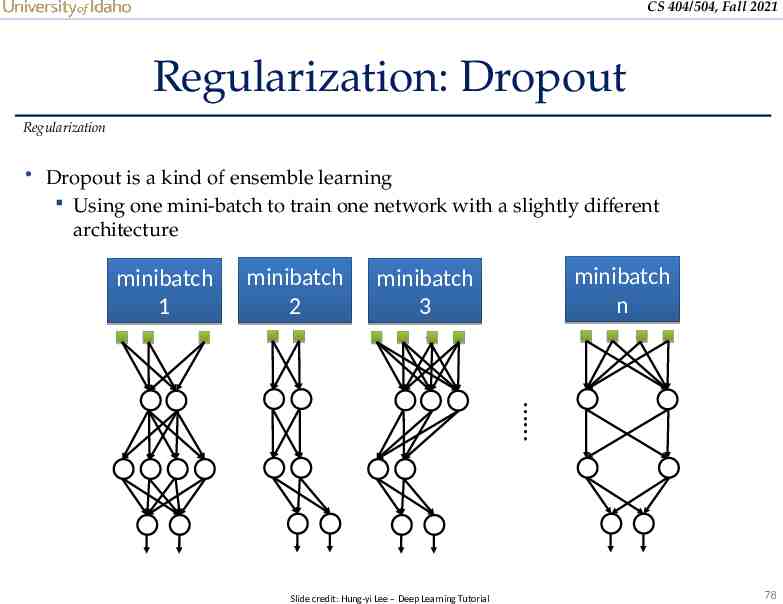
CS 404/504, Fall 2021 Regularization: Dropout Regularization Dropout is a kind of ensemble learning Using one mini-batch to train one network with a slightly different architecture minibatch 1 minibatch 2 minibatch n minibatch 3 Slide credit: Hung-yi Lee – Deep Learning Tutorial 78
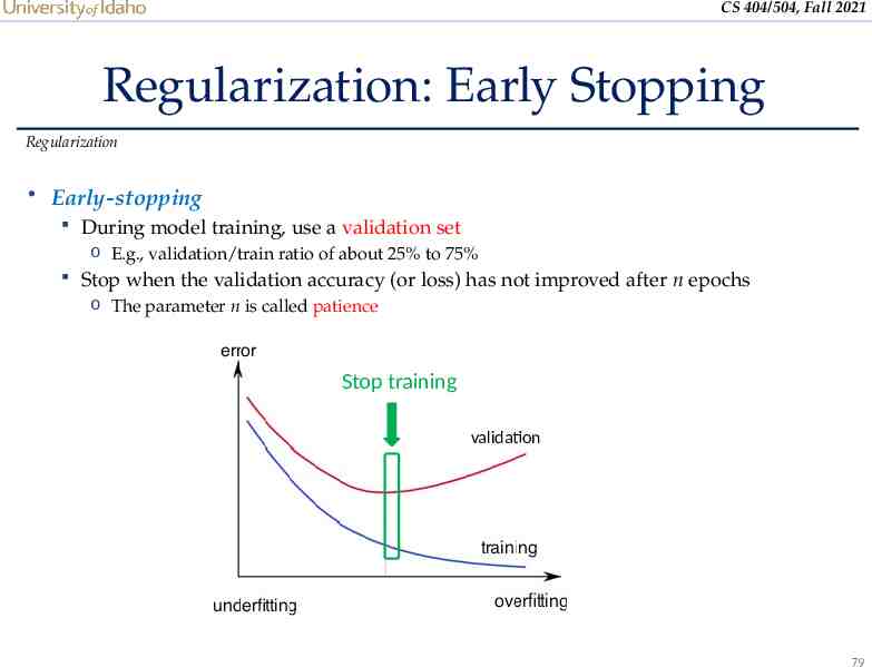
CS 404/504, Fall 2021 Regularization: Early Stopping Regularization Early-stopping During model training, use a validation set o E.g., validation/train ratio of about 25% to 75% Stop when the validation accuracy (or loss) has not improved after n epochs o The parameter n is called patience Stop training validation 79
CS 404/504, Fall 2021 Batch Normalization Regularization Batch normalization layers act similar to the data preprocessing steps mentioned earlier They calculate the mean μ and variance σ of a batch of input data, and normalize the data x to a zero mean and unit variance I.e., BatchNorm layers alleviate the problems of proper initialization of the parameters and hyper-parameters Result in faster convergence training, allow larger learning rates Reduce the internal covariate shift BatchNorm layers are inserted immediately after convolutional layers or fully- connected layers, and before activation layers They are very common with convolutional NNs 80
CS 404/504, Fall 2021 Hyper-parameter Tuning Hyper-parameter Tuning Training NNs can involve setting many hyper-parameters The most common hyper-parameters include: Number of layers, and number of neurons per layer Initial learning rate Learning rate decay schedule (e.g., decay constant) Optimizer type Other hyper-parameters may include: Regularization parameters ( penalty, dropout rate) Batch size Activation functions Loss function Hyper-parameter tuning can be time-consuming for larger NNs 81
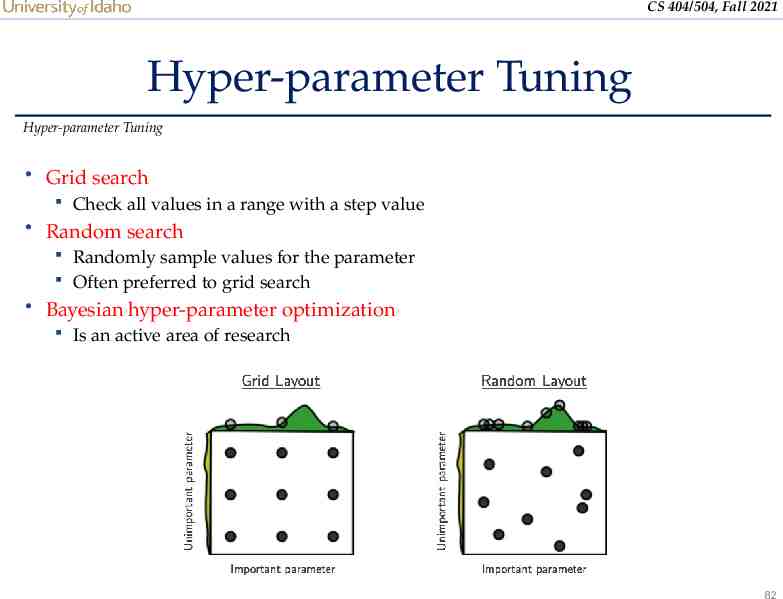
CS 404/504, Fall 2021 Hyper-parameter Tuning Hyper-parameter Tuning Grid search Check all values in a range with a step value Random search Randomly sample values for the parameter Often preferred to grid search Bayesian hyper-parameter optimization Is an active area of research 82
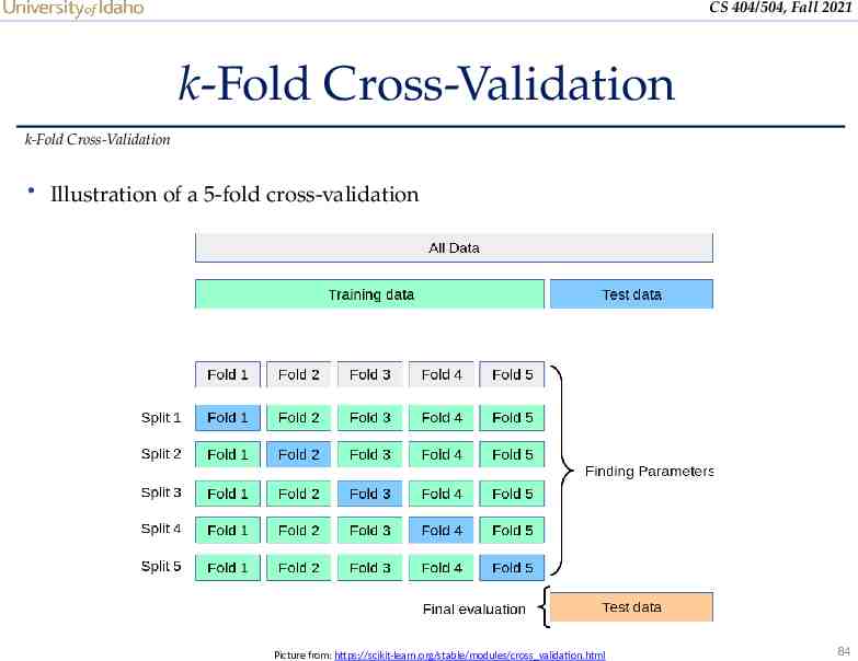
CS 404/504, Fall 2021 k-Fold Cross-Validation k-Fold Cross-Validation Using k-fold cross-validation for hyper-parameter tuning is common when the size of the training data is small It also leads to a better and less noisy estimate of the model performance by averaging the results across several folds E.g., 5-fold cross-validation (see the figure on the next slide) 1. Split the train data into 5 equal folds 2. First use folds 2-5 for training and fold 1 for validation 3. Repeat by using fold 2 for validation, then fold 3, fold 4, and fold 5 4. Average the results over the 5 runs (for reporting purposes) 5. Once the best hyper-parameters are determined, evaluate the model on the test data 83
CS 404/504, Fall 2021 k-Fold Cross-Validation k-Fold Cross-Validation Illustration of a 5-fold cross-validation Picture from: https://scikit-learn.org/stable/modules/cross validation.html 84
CS 404/504, Fall 2021 Ensemble Learning Ensemble Learning Ensemble learning is training multiple classifiers separately and combining their predictions Ensemble learning often outperforms individual classifiers Better results obtained with higher model variety in the ensemble Bagging (bootstrap aggregating) o Randomly draw subsets from the training set (i.e., bootstrap samples) o Train separate classifiers on each subset of the training set o Perform classification based on the average vote of all classifiers Boosting o Train a classifier, and apply weights on the training set (apply higher weights on misclassified examples, focus on “hard examples”) o Train new classifier, reweight training set according to prediction error o Repeat o Perform classification based on weighted vote of the classifiers 85
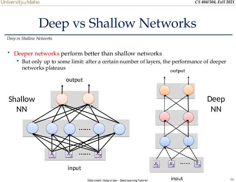
CS 404/504, Fall 2021 Deep vs Shallow Networks Deep vs Shallow Networks Deeper networks perform better than shallow networks But only up to some limit: after a certain number of layers, the performance of deeper networks plateaus output Deep NN Shallow NN x1 x2 xN input Slide credit: Hung-yi Lee – Deep Learning Tutorial 86
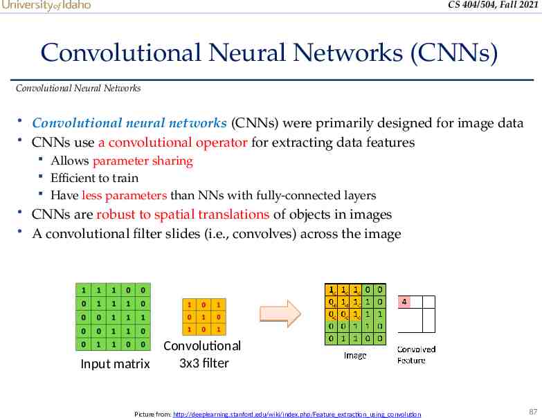
CS 404/504, Fall 2021 Convolutional Neural Networks (CNNs) Convolutional Neural Networks Convolutional neural networks (CNNs) were primarily designed for image data CNNs use a convolutional operator for extracting data features Allows parameter sharing Efficient to train Have less parameters than NNs with fully-connected layers CNNs are robust to spatial translations of objects in images A convolutional filter slides (i.e., convolves) across the image Input matrix Convolutional 3x3 filter Picture from: http://deeplearning.stanford.edu/wiki/index.php/Feature extraction using convolution 87
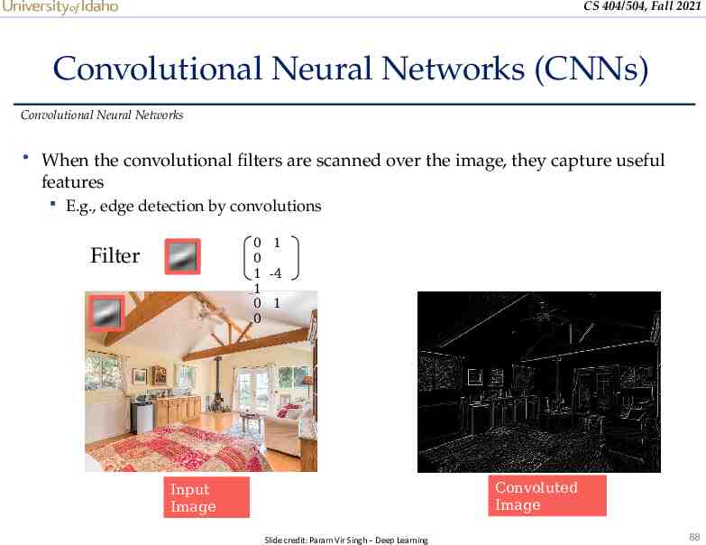
CS 404/504, Fall 2021 Convolutional Neural Networks (CNNs) Convolutional Neural Networks When the convolutional filters are scanned over the image, they capture useful features E.g., edge detection by convolutions 0 1 0 1 -4 1 1 1 1 0.015686 0.015686 0.011765 0.015686 0.015686 0.015686 0.015686 0.964706 0.988235 0.964706 0.866667 0.031373 0.023529 0.007843 1 0.984314 0.023529 0.019608 0.015686 0.015686 0.015686 0.011765 0.101961 0.972549 1 0 1 0.996078 0.996078 1 0.996078 0.058824 0.015686 1 1 0.019608 0.015686 0.015686 0.015686 0.007843 0.011765 1 1 1 0.996078 0.031373 0.015686 0.019608 1 0.011765 00.015686 0.007843 0.007843 1 0.352941 1 0.996078 0.019608 0.019608 0.015686 0.015686 0.011765 0.984314 1 1 0.988235 0.027451 Filter 1 1 1 0.007843 0.741176 1 0.019608 0.513726 1 0.015686 0.733333 1 0.015686 0.823529 1 1 0.988235 0.019608 0.019608 0.015686 0.015686 0.019608 1 1 0.980392 0.015686 0.015686 0.015686 0.015686 0.996078 1 0.996078 0.015686 0.913726 1 1 0.996078 0.019608 0.019608 0.019608 0.019608 1 1 0.984314 0.015686 0.015686 0.015686 0.015686 0.952941 1 1 0.992157 0.019608 0.913726 1 1 0.988235 0.019608 0.019608 0.019608 0.039216 0.996078 1 0.015686 0.015686 0.015686 0.015686 0.996078 1 1 1 0.007843 0.019608 0.898039 1 1 0.988235 0.019608 0.015686 0.019608 0.968628 0.996078 0.980392 0.027451 0.015686 0.019608 0.980392 0.972549 1 1 1 0.019608 0.043137 0.905882 1 1 1 0.015686 0.035294 0.968628 1 1 0.023529 1 0.792157 0.996078 1 1 0.980392 0.992157 0.039216 0.023529 1 1 1 1 1 0.992157 0.992157 1 1 0.984314 0.015686 0.015686 0.858824 0.996078 1 0.992157 0.501961 0.019608 0.019608 0.023529 0.996078 0.992157 1 1 1 0.933333 0.003922 0.996078 1 0.988235 1 0.992157 1 1 1 0.988235 1 1 1 1 0.015686 0.74902 1 1 0.984314 0.019608 0.019608 0.031373 0.984314 0.023529 0.015686 0.015686 1 1 1 0 0.003922 0.027451 0.980392 1 0.019608 0.023529 1 1 1 0.019608 0.019608 0.564706 0.894118 0.019608 0.015686 0.015686 1 1 1 0.015686 0.015686 0.015686 0.05098 1 0.015686 0.015686 1 1 1 0.047059 0.019608 0.992157 0.007843 0.011765 0.011765 0.015686 1 1 1 0.015686 0.019608 0.996078 0.023529 0.996078 0.019608 0.015686 0.243137 1 1 0.976471 0.035294 1 0.003922 0.011765 0.011765 0.015686 1 1 1 0.988235 0.988235 1 0.003922 0.015686 0.019608 0.019608 0.027451 1 1 0.992157 0.223529 0.662745 0.011765 0.011765 0.011765 0.015686 1 1 1 0.015686 0.023529 0.996078 0.011765 0.011765 0.015686 0.015686 0.011765 1 1 1 1 0.035294 0.011765 0.011765 0.011765 0.015686 1 1 1 0.015686 0.015686 0.964706 0.003922 0.996078 0.007843 0.019608 0.011765 0.054902 1 1 0.988235 0.007843 0.011765 0.011765 0.015686 0.011765 1 1 1 0.015686 0.015686 0.015686 0.023529 1 0.007843 0.007843 0.015686 0.015686 0.960784 1 0.490196 0.015686 0.015686 0.015686 0.007843 0.027451 1 1 1 0.011765 0.011765 0.043137 1 1 0.023529 0.003922 0.007843 0.023529 0.980392 0.976471 0.039216 0.019608 0.007843 0.019608 0.015686 1 1 1 1 1 1 1 1 1 Convoluted Image Input Image Slide credit: Param Vir Singh – Deep Learning 88
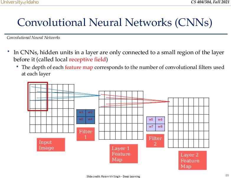
CS 404/504, Fall 2021 Convolutional Neural Networks (CNNs) Convolutional Neural Networks In CNNs, hidden units in a layer are only connected to a small region of the layer before it (called local receptive field) The depth of each feature map corresponds to the number of convolutional filters used at each layer Input Image w1 w2 w3 w4 Filter 1 Layer 1 Feature Map Slide credit: Param Vir Singh – Deep Learning w5 w6 w7 w8 Filter 2 Layer 2 Feature Map 89
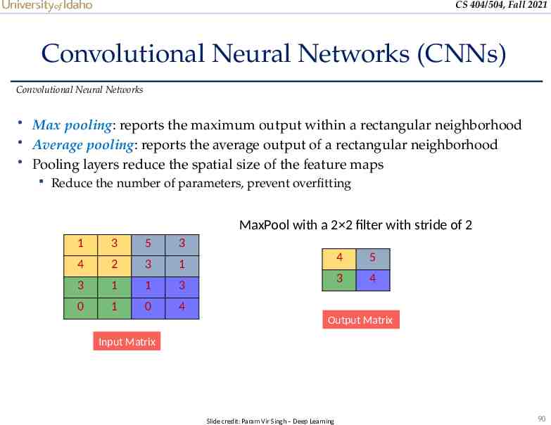
CS 404/504, Fall 2021 Convolutional Neural Networks (CNNs) Convolutional Neural Networks Max pooling: reports the maximum output within a rectangular neighborhood Average pooling: reports the average output of a rectangular neighborhood Pooling layers reduce the spatial size of the feature maps Reduce the number of parameters, prevent overfitting MaxPool with a 2 2 filter with stride of 2 1 3 5 3 4 2 3 1 3 1 1 3 0 1 0 4 4 5 3 4 Output Matrix Input Matrix Slide credit: Param Vir Singh – Deep Learning 90
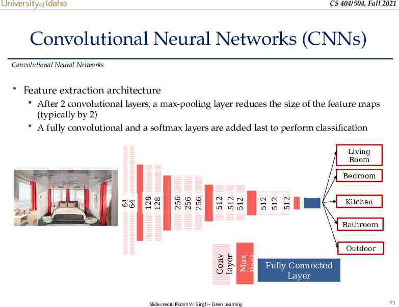
CS 404/504, Fall 2021 Convolutional Neural Networks (CNNs) Convolutional Neural Networks Feature extraction architecture After 2 convolutional layers, a max-pooling layer reduces the size of the feature maps (typically by 2) A fully convolutional and a softmax layers are added last to perform classification Living Room 512 512 512 512 512 512 256 256 256 128 128 Kitchen Bathroom Max Pool Outdoor Conv layer 64 64 Bedroom Slide credit: Param Vir Singh – Deep Learning Fully Connected Layer 91
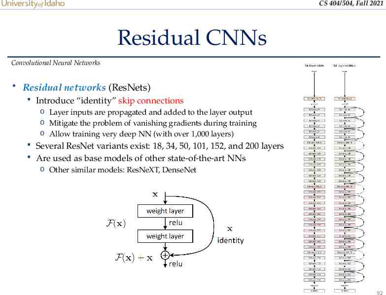
CS 404/504, Fall 2021 Residual CNNs Convolutional Neural Networks Residual networks (ResNets) Introduce “identity” skip connections o Layer inputs are propagated and added to the layer output o Mitigate the problem of vanishing gradients during training o Allow training very deep NN (with over 1,000 layers) Several ResNet variants exist: 18, 34, 50, 101, 152, and 200 layers Are used as base models of other state-of-the-art NNs o Other similar models: ResNeXT, DenseNet 92
CS 404/504, Fall 2021 Recurrent Neural Networks (RNNs) Recurrent Neural Networks Recurrent NNs are used for modeling sequential data and data with varying length of inputs and outputs Videos, text, speech, DNA sequences, human skeletal data RNNs introduce recurrent connections between the neurons This allows processing sequential data one element at a time by selectively passing information across a sequence Memory of the previous inputs is stored in the model’s internal state and affect the model predictions Can capture correlations in sequential data RNNs use backpropagation-through-time for training RNNs are more sensitive to the vanishing gradient problem than CNNs 93
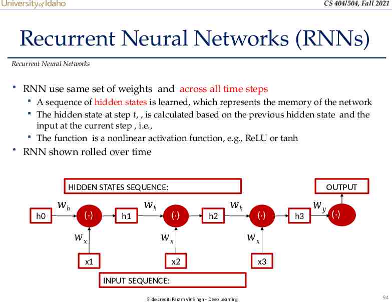
CS 404/504, Fall 2021 Recurrent Neural Networks (RNNs) Recurrent Neural Networks RNN use same set of weights and across all time steps A sequence of hidden states is learned, which represents the memory of the network The hidden state at step t, , is calculated based on the previous hidden state and the input at the current step , i.e., The function is a nonlinear activation function, e.g., ReLU or tanh RNN shown rolled over time HIDDEN STATES SEQUENCE: 𝑤h h0 (·) 𝑤𝑥 𝑤h OUTPUT (·) h1 𝑤h h2 𝑤𝑥 x1 x2 (·) h3 𝑤𝑦 (·) 𝑤𝑥 x3 INPUT SEQUENCE: Slide credit: Param Vir Singh – Deep Learning 94
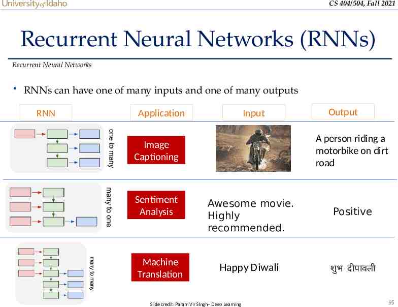
CS 404/504, Fall 2021 Recurrent Neural Networks (RNNs) Recurrent Neural Networks RNNs can have one of many inputs and one of many outputs RNN Application Input A person riding a motorbike on dirt road Image Captioning Sentiment Analysis Machine Translation Output Awesome movie. Highly recommended. Positive Happy Diwali शुभ दीपावली Slide credit: Param Vir SIngh– Deep Learning 95
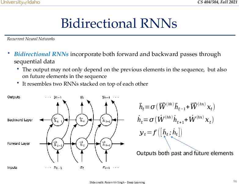
CS 404/504, Fall 2021 Bidirectional RNNs Recurrent Neural Networks Bidirectional RNNs incorporate both forward and backward passes through sequential data The output may not only depend on the previous elements in the sequence, but also on future elements in the sequence It resembles two RNNs stacked on top of each other (hh) (h𝑥) ⃑h𝑡 𝜎 ( ⃑ 𝑊 h⃑ 𝑡 1 ⃑ 𝑊 𝑥𝑡 ) (hh) h́ 𝑊 (h𝑥) 𝑥 ) h́𝑡 𝜎 ( 𝑊 𝑡 1 𝑡 𝑦𝑡 𝑓 ( [ ⃑h𝑡 ; h́𝑡 ] ) Outputs both past and future elements Slide credit: Param Vir Singh – Deep Learning 96
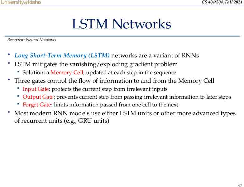
CS 404/504, Fall 2021 LSTM Networks Recurrent Neural Networks Long Short-Term Memory (LSTM) networks are a variant of RNNs LSTM mitigates the vanishing/exploding gradient problem Solution: a Memory Cell, updated at each step in the sequence Three gates control the flow of information to and from the Memory Cell Input Gate: protects the current step from irrelevant inputs Output Gate: prevents current step from passing irrelevant information to later steps Forget Gate: limits information passed from one cell to the next Most modern RNN models use either LSTM units or other more advanced types of recurrent units (e.g., GRU units) 97
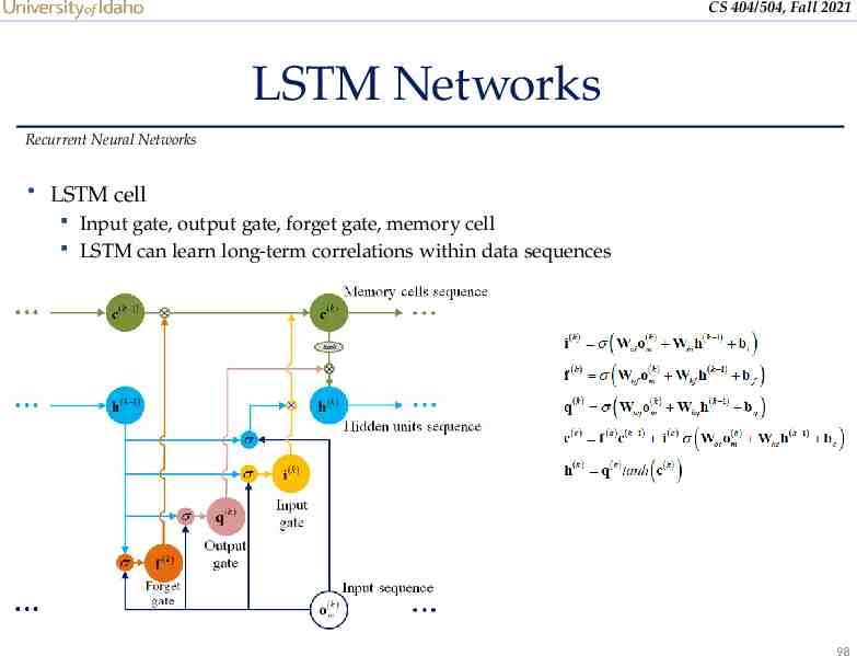
CS 404/504, Fall 2021 LSTM Networks Recurrent Neural Networks LSTM cell Input gate, output gate, forget gate, memory cell LSTM can learn long-term correlations within data sequences 98
CS 404/504, Fall 2021 References 1. 2. 3. 4. 5. 6. Hung-yi Lee – Deep Learning Tutorial Ismini Lourentzou – Introduction to Deep Learning CS231n Convolutional Neural Networks for Visual Recognition (Stanford CS course) (link) James Hays, Brown – Machine Learning Overview Param Vir Singh, Shunyuan Zhang, Nikhil Malik – Deep Learning Sebastian Ruder – An Overview of Gradient Descent Optimization Algorithms (link) 99